Spring Batch: making massive batch processing on Java

Standard

Welcome, dear reader, to another post from my technology blog. In this post, we discuss a framework that may not be very familiar to everyone, but it is a very powerful feature in the construction of batch applications made in Java: The Spring Batch.

Batch Application: what it is

A batch application, in general, is nothing more than a program whose goal is to make the processing of large amounts of data, on a scheduled basis, usually through programmed trigger mechanisms (scheduling).

Typically, on companies, we see many such programs been built directly into the database layer, using languages such as PL \ SQL, for example. This method has its advantages, but there are several advantages that can draw to build a batch program in a technology like Java. One advantage we get is the ease of application scalation, as a batch built in this language will typically run as a standalone program or within an application server, so you can have your memory, CPU, etc more easily scaled than the alternative of a batch in PL \ SQL. Moreover, the alternative of making a batch on Java offers more opportunities of reuse, as the same logic can be applied to  batch, web, REST, etc.

So, having made our introduction to the subject, let’s proceed and start talking about the framework.

Framework architecture

In the figure below, taken from the framework documentation, can we see the main components that make up the architecture of a Spring Batch job. Let’s see in better detail.


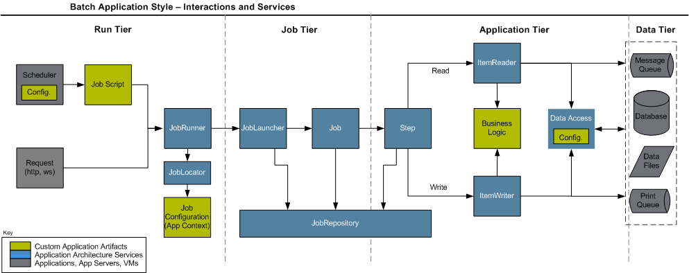
As we can see above, when we build a job – a term commonly used to describe a batch program, we will use from now – in the framework, you must implement three types of artifacts: a job script, which consists of an implementation plan with steps, which makes up the job execution, connection settings for the data sources that the job will process such as databases, JMS queues, etc. and of course, classes that implement the processing logic.

When we use the framework for the first time, a step of the setup is to create a set of database tables, whose function is to provide the basis for a repository of jobs. The framework focuses on the concept where you can, through these tables, control the status of different jobs, through the different executions, allowing a restartability mechanism, that is, it allows a job to be restarted from the point at which it stopped in the last run, in case of failure. To achieve this control, the Spring Batch provides the following control structure represented by a set of classes:

JobRunner: Class responsible to make the execution of a job by external request. Has several implementations to provide method invocation call for different modes such as a shell script, for example. Performs the instantiation of a JobLauncher;

JobLocator: Class responsible for getting the configuration information, such as the implementation plan (job script), for a given job passed by parameter. Works in conjunction with the JobRunner;

JobLauncher: Class responsible for managing the start and manage the actual execution of the job, is instantiated by JobRunner;

JobRepository: Facade class that interface the access of the framework classes to the tables of the repository, it is through this class that jobs communicate the progress of its executions, thus ensuring that it could make his restart;

Thanks to this mechanism of control, Spring provides a web application, developed in Java, which allows actions like view execution logs of batches and start / stop / restart jobs through the interface, called Spring Batch Admin. More information about the application can be found at the end of the post.

Now that we have clarified the framework architecture, let’s talk about the main components (classes / interfaces that the developer must implement) that the developer has at his disposal for the construction of the processing logic itself.

Components

Tasklet: Basic unit of a step, can be created for the development of specific actions of the batch, like calling a webservice which data is to be used for all steps of the implementation, for example.

ItemReader: Component used in a structure known as chunk, where we have a data source that is read, processed and written in an iterative fashion, into blocks – chunks – until all the data has been processed. This component is the logic of reading, that read sources such as databases. The framework comes with a set of pre-build readers, but the developer can also develop your own if necessary.

ItemProcessor: Component used in a structure known as chunk, where we have a data source that is read, processed and written in an iterative fashion, into blocks – chunks – until all the data has been processed. This component is the processing logic, which typically consists of the execution of business rules, calls to external resources for enrichment of data, such as web services, among others.

ItemWriter: Component used in a structure known as chunk, where we have a data source that is read, processed and written in an iterative fashion, into blocks – chunks – until all the data has been processed. This component is for the writte logic of the processed data, like with the ItemReaders, the framework also comes with a set of pre-build ItemWriters to write on sources such as databases, but the developer can also develop your own writer, if necessary.

Decider: Component responsible for making use of logic to perform tasks like “go to the step 1 if a value equal to X, if equal to Y go to the step 2, and ends the execution if the value is equal to Z “.

Classifier: Component that can be used in conjunction with other components, such as a ItemWriter and perform classification logic, such as “run ItemWriterA for the item if it has the property X = true, otherwise, execute the ItemWriterB “. IMPORTANT: IN THIS SCENARIO, THE ORDER OF EXECUTION OF THE ITEMS WITHIN THE CHUNK IS MODIFIED, BECAUSE THE FRAMEWORK  MAKES ALL THE CLASSIFICATION OF THE ITEMS FIRST, AND THEN EXECUTE 1 ITEMWRITER AT A TIME!

Split: Component used when you want, at a certain point of execution, a set of steps to run in parallel through multithreading.

About the Java EE 7 Batch specification

Some readers may be familiar with the new API called “Batch”, the JSR-352, which introduces a new batch processing API in Java EE 7 platform, having very similar concepts to Spring Batch, it fills an important gap in the implementation of reference of the Java technology. More than a philosophical question, some attention points should be considered before you choose to use one or the other framework, such as the requirement of a Java EE container (server) for its implementation, the lack of support for the use via jdbc in access to the databases, and the absence of support for reading outsourced properties in files, which the Spring Batch can use through components called PropertyPlaceHolders. In the links at the end of the post, you can read an article detailing the differences of the two in more depth.

Conclusion

Unfortunately, you can not detail, in a single post, all the power of the framework. Several things were left out, such as support for event listeners in the execution of jobs, error treatments allowing certain exceptions have retries policies or being “ignored” (retry, skip), among other features. I hope, however, be transmitted to the reader a good initial view of the framework, sharpening his curiosity. Massive data processing has always been, and always will be a major challenge for companies, and our mission, as IT professionals, is the constant learning of the best resources we have available. Thank you for your attention, and until next time.

Continue reading

Hands-on: DevOps with Vagrant

Standard

Welcome to another post of my blog. In this post, we’ll talk about a topic widely spoken in the midst of IT in recent times, called DevOps.

DevOps: what it is

Speaking in general terms, DevOps is a new way to integrate the work among software development teams and operating teams (Production) that support software. Through tools that make the act of starting / end servers, install / uninstall packages, configure servers and deploy software updated quick and automated, we have an IT environment where changes can be deployed into production more quickly and to a lesser granularity – by delivering less features – which becomes also lower the risk of impact on the production environment.

For this hands-on, we will use one of the most popular technologies DevOps have, Vagrant, along with Puppet. The function of Vagrant is to make the start, stop and / or restart of servers, while the Puppet is responsible for making the necessary settings on the servers, such as the rise of application servers – JBoss, etc. – port configuration and threshoulds memory, among other actions. For the hands-on, we used the ubuntu 14:04.

Installing Vagrant

The installation of Vagrant is quite simple and fast. First, we have to install VirtualBox, which is the virtualization technology used by default by Vagrant. For that, on the Ubuntu command prompt, type the following command:

sudo apt-get install virtualbox

After running the command – remember to enter “Y” (yes) when the prompt request – virtualbox will be installed on the OS. Next, you must install Vagrant, using the following command:

sudo apt-get install vagrant

After running the command, the last two configuration steps for the Virtualbox are necessary because it uses OS kernel modules that are not loaded by default. To perform the configuration, run the two commands below in sequence:

sudo apt-get install linux-headers-$(uname -r)

sudo dpkg-reconfigure virtualbox-dkms

After running these commands, the installation is complete.

Starting with Vagrant

Within the Vagrant pattern for the creation of servers, we have the concept of boxes. Through the boxes, you can create a basic server with an OS already installed, instead of performing all zero configuration. For this hands-on, we will use a 32-bit ubuntu 12  box, also called “precise”. To add a box, run the following command:

vagrant box add precise32 http://files.vagrantup.com/precise32.box

After downloading and including the box, the next step is to initialize the Vagrant with the box. To do this, navigate the terminal to a folder of your choice – in my example, I created a “vagrant” folder within my desktop and moved the terminal there – and enter the following command:

vagrant init precise32

After running the command, the reader will notice that was created in the folder chosen a file called “Vagrantfile”. This file is the central file, where the servers are set to be deployed. We will demonstrate this hands-on with a simple example, where it will be created a machine with a tomcat server. To begin, let’s create two folders at the same level of the file “vagrantfile”, called “modules” and “manifests”. In the main file, “vagrantfile”, insert the following code:

VAGRANTFILE_API_VERSION = “2”

Vagrant.configure(VAGRANTFILE_API_VERSION) do |config|
config.vm.box = “hashicorp/precise32”

config.vm.define :web do |web_config|
web_config.vm.network :private_network, :ip => “192.168.33.12”
web_config.vm.provision “puppet” do |puppet|
puppet.module_path = “modules”
puppet.manifest_file = “web.pp”
end
end

end

As shown above, the code configured version of Vagrant API that we will use, the box used, and set up a machine to be started using the box on the ip “192.168.33.12”. In addition, we set the folder modules, which we’ll discuss later, and the name of the provisioning file, of .pp extension. This file has instructions for Puppet to perform the settings on the machine, as in our case, will perform the installation and rise of the Tomcat. Before we see the Puppet file, we will discuss the concept of modules within the Puppet.

Puppet modules

Within Puppet, we have the concept of modules. A Puppet module can be explained as something analogous to a class in the OO paradigm, where classes and methods that encapsulate the configuration commands are defined, so that it is not necessary to repeat the provisioning code to each newly created Puppet project. In the puppet forge there are several modules ready and made available by the community. For this hands-on, we will use the modules of the links below:

https://forge.puppetlabs.com/puppetlabs/stdlib

https://forge.puppetlabs.com/puppetlabs/apt

PS: For this hands-on, we are not using the Vagrant plugin called librarian, in order to maintain the most simple and compact explanation. In a similar manner with other dependency management technologies such as maven, the librarian manages dependencies of Puppet modules. The reader can find a link to the project page on GitHub in the section read more.

The above modules consist of a module of basic utility functions of the Puppet (“stdlib”) and basic functions of OS (“apt”) as “apt-update sudo”. To manually install the modules, download the same as a tar.gz file and unpack them in the “modules” folder. After extracting the files, adjust the names of the modules by removing the prefix and the version, for example by modifying the “puppetlabs-apt-1.6.0” to “apt”. At the end of this post, I will provide a link  with all the necessary files and modules.

Finally, we have the puppet file below, which makes server provisioning:

class { ‘apt’:
always_apt_update => true,
}

Class[‘apt’] -> Package <| |>

Exec {
path => ‘/usr/bin:/usr/sbin/:/bin:/sbin:/usr/local/bin:/usr/local/sbin’,
}

package { [“tomcat7”]:
ensure => installed,
}

service { “tomcat7”:
ensure => running,
enable => true,
hasstatus => true,
hasrestart => true,
require => Package[“tomcat7”],
}

This file should be saved as “web.pp” and saved in the folder “manifests” .In the above code, we make the following sequence of actions: We created an apt class, stating that it must perform an apt-update (“always_apt_update “). On the next line, we indicate that the command should be run whenever a package is installed. In the following lines, we set the package installation tomcat7, perform the startup, and set an OS service for the same.

To start the server with provisioning, run the following command in the command prompt:

vagrant up

The result, when we put the address 192.168.33.12:8080, that is, the ip we set for the machine, and the default port of the tomcat server, is the welcome screen of the server, as can be seen below:

successTo stop the server, simply run the command “vagrant suspend”. With the command “vagrant destroy”, not just the server is stopped, but the instance is also destroyed. The full list of vagrant commands can be found in the links section read more.

Conclusion

In this post we had a brief introduction of the concept of DevOps and the Vagrant technology. With an intuitive language and easy to maintain, it allows us to automate complex infrastructure operations, thereby facilitating the “fearful” process of deploying applications in the production environment. As a concept still growing, it may take some time for the market as a whole to adopt his philosophy, but without a doubt, has many benefits for IT processes within companies.

Continue reading

Big Data – part 3

Standard

In this post we will proceed to our series on Big Data. If the reader has not read the previous posts in this series, the links can be found at the end of this post, or the menus, “Big Data” section.

In this post, we will discuss one of the most popular technologies of the moment in the development of Big Data solutions: Apache Hadoop.

Origin

Hadoop was created in 2005 by two developers, Doug Cutting and Mike Cafarella. The symbol of Hadoop, the famous yellow elephant, it is Mike’s son toy elephant, and the name “Hadoop” is the elephant’s name. In the video below we can see the co-creator in an interview, talking about the challenges of data mining:

Architecture

Speaking of the Hadoop architecture, we can separate into 2 main parts, consisting of two clusters:

  1. One part consists of a cluster that implements a distributed file system, known as HDFS (Hadoop Distributed File System);
  2. The second part consists of another cluster, which provides an environment for executing programs written following the MapReduce model. If the reader does not know what is mapreduce, we address this point in Part 2 of our series;

Lets examine, in general, each of these clusters:

HDFS

The HDFS, Hadoop file storage system consists of a system that allows files to be stored across multiple nodes (servers). When we insert a file in the cluster, either through the command line interface and / or its REST interface, or when we have mapreduce processes generating processing of output files, the HDFS makes a “break” of the file into several smaller files – by default, parts of 64MB – and distributes the files across the nodes, managing details on run time as the number of copies that each part must have, remaking this balancing in case of a cluster node falls. All this break is transparent to the developer because the cluster will make the mounting in every query made through the interfaces.

A HDFS cluster consists of two components:

  1. NameNodes: Central cluster component, responsible for managing the assembly metadata – used to reconstruct the original files – and make the management of the files in the cluster;
  2. DataNodes: “Physical” component of the cluster, responsible for making the read / write of the files on the disk. Each node has its DataNode, which performs the read / write on the server disk that is running;

PS: Na versão 2.0 do Hadoop, um novo componente foi incluso no HDFS, chamado YARN (Yet Another Resource NameNode), cujo objetivo principal é fornecer uma camada a mais de interface entre os usuários do HDFS e o mesmo. Graças a essa melhoria, podemos ter no cluster também diversos NameNodes para efetuar o gerenciamento dos arquivos, evitando assim o problema da possível perda de um cluster HDFS no caso de problemas irrecuperáveis com os NameNodes, como no caso do Hadoop 1.0, onde tinhamos, tipicamente, apenas dois processos de NameNode, sendo um deles para mecanismo de failover.

Mapreduce cluster

The mapreduce cluster  consists of a cluster which performs the execution of mapreduce processes. Typically, the input / output of a mapreduce job in Hadoop is with HDFS using the NameNode (YARN in version 2.0) to interface the cluster with the HDFS. The following are the components of a  MapReduce cluster:

  1. JobTracker: Component that interface the cluster with the developers, makes the management of process execution, identifying with the NameNode from the HDFS cluster where each part of the input data is to be processed, indicating for TaskTrackers which part of the data to process, and manages the beginning and end of each stage of processing;
  2. TaskTracker:Component that receives from the JobTracker the instructions for executing jobs, which parts of the mass of data it is responsible for processing, and report to the JobTracker when processing is complete;
  3. Task: Smaller cluster unit, the Task is responsible for making the processing itself. Each task can be performed in a JVM instance initiated during process execution, or it can be instantiated in a JVM already started with other Tasks running, according to the specified memory consumption settings in the cluster;

Hadoop complementary software

Several software was created to complement the use of Hadoop, or even built from the same. A brief description of some of them:

  • Mahout: Allows you to use machine learning techniques for data analysis in hadoop;
  • Sqoop: Allows integrate HDFS with relational databases;
  • Hive: Allows consultations in HDFS more easy way, through SQL commands;
  • Hama: Allow the development of jobs in Hadoop on other models besides the mapreduce, as the BSP;
  • HBase: NoSQL database, built under the HDFS;

In future posts, we will discuss this software in more detail.

Conclusion

And so, we concluded one more post of our series. With the growth of projects and solutions in Big Data worldwide, the hadoop has grown a lot as a market-leading technology, already having market implementations of large players like Cloudera and Hortonworks. In the next post, we will address other well known technology in the world of Big Data: the Spark. Until next time.

Continue reading

Raspberry PI – Entering the world of embedded software

Standard

In this post, we will discuss a first look at the Raspberry PI and a macro view of what’s embedded software. We’ll start by answering the following question: but after all, what is a Raspberry PI?

A computer the size of a credit card

The Raspberry PI it is a laptop, or in other words an integrated circuit board containing several features such as audio, video, network – the standard version of the board does not have support for wi-fi – the size of a card credit. Developed in the UK, its main goal is to provide a means for computer science learning in schools, and allows the development of solutions involving the combination software + hardware, such as home automation, monitoring systems for security, etc.

Currently, the card is sold in two designs, known as A and B:

especs_pi

Source: Wikipedia

As we can see in the specifications, it is a very powerful processing power, considering its dimensions. Some features of the board, such as the camera and the wifi, is not available from the factory, so it is necessary to buy separately the official accessories, or use the GPIO interface (which we will discuss later) to connect the card to additional circuits such as sensors, alarms or even electronic circuits that you can build yourself!

A  B model raspberry pi

Operational system

The standard operating system of the card is the raspbian, a Debian distribution made especially for the card. The OS installation procedure on the SD card is quite simple and can be learned in the tutorial video below:

Embedded Software

The concept of embedded software, is of programs that run on low-cost and / or hardware resources, usually for projects involving the automation of processes of the physical world, as controls closing doors with motion detection, curtains that open and close according to the brightness of a room, fire detectors and so on. On this site you can see several projects made with the raspberry pi. There´s even drones!

The raspberry pi due to have a complete operating system, with all the basic features of a desktop operating system, allows to use different programming languages such as Python, Ruby, and even Java. In my experiences with the card, I recommend using Python, due to have a more complete support in many ways, as a good library for handling the GPIO.

GPIO

The GPIO – General Purpose IO – consists of a set of electronic pins which provide input, output and ground for the connection of other electronic components to the pi. The figure below shows the layout of the pins, in a future post, we’ll talk specifically about this interface.

Shops

From my experiences on my country (Brazil), this are the best shops to buy eletronic components and the PI itself, so I recommend:

Lab de garagem

Farnell Newark

Multi Comercial (loja da Santa Efigênia)

Conclusion

And so we conclude our first general contact with the world of embedded software, and raspberry pi. In future posts, we will deepen more on the many issues that we brushed on the post. Until next time.

Big Data – part 2

Standard

This is the second part of a series of posts on Big Data.On this post, let’s talk about the two most popular distributed  processing models of Big Data, the mapreduce, and the BSP (Bulk Synchronous Parallel). A process model is a kind of algorithm upon which to develop software.

Mapreduce model

Modelo map reduce

In the figure above, we can see the mapreduce model. This model is widely used in the market today, especially in companies that use Hadoop as her main Big Data technology. The model consists of two well-defined steps, called map and reduce:

  • In the step known as Map, hundreds – or even thousands – of parallel processes, called “threads”, perform a type of task called mapping, where a large mass of data is divided into pieces, and each performs a filtering process within a respective piece, creating a mass of values in the key-value format. At the end of this phase, there is a group phase, where the values for the same key are grouped to form data in the format key: {value1, value2, value3 …. valueN};
  • In the step known as reduce, the data generated by the map phase is again divided into pieces and passed to hundreds or even thousands of processes that perform processing on the received data bits and generate as a key-value output, which is the final output of the processing that is finally grouped into a mass of results;

In a future post, we’ll take a hands-on hadoop, where we can see an example of this processing model in practice with the WordCount.

BSP Model (Bulk Synchronous Parallel)

bsp

Although widespread, the mapreduce model is not without its drawbacks. When we talk about the model being applied in the context of Hadoop, for example, all of the cluster steps and mounting of the final mass with the results is done through files on the file system of Hadoop, HDFS, which generates an overhead in performance when it has to perform the same processing in a iterative manner.Another problem is that for graph algorithms such as DFS, BFS or Pert, MapReduce model is not satisfactory. For these scenarios, there is the BSP.

In the BSP algorithm, we have the concept of supersteps. A superstep consists of a unit of generic programming, which through a global communication component, makes thousands of parallel processing on a mass of data and sends it to a “meeting” called synchronization barrier. At this point, the data are grouped, and passed on to the next superstep chain. In this model, it is simpler to construct iterative workloads, since the same logic can be re-executed in a flow of supersteps. Another advantage pointed out by proponents of this model is that it has a simpler learning curve for developers coming from the procedural world.

Speaking in terms of platforms, Hadoop has the Apache Hama as implementation of this model. The main competitor of Hadoop, Spark, come with this feature natively.

Conclusion

And so we conclude another part of our series on Big Data. To date, these are the main models used by the Big Data platforms. As a technology booming, it is natural that in the future we could have more models emerging and gaining their adoption shares. In the next parts of our series, we’ll talk about the two most known implementations of Big Data to date: Hadoop and Spark. U.

Continue reading

Hands-on: JSON Java API

Standard

JSON (JavaScript Object Notation) is a notation for data communication, as well as XML, for example. Its popularity has grown with the growth of the REST Web Services, and today has long been used in the development of APIs.

In this hands-on, we will learn how to use a JSON Java API, present in Java EE 7. With it, you can parse JSON structures for reading the data, and generate their own structures.

Creating the project

In this hands-on we will use Eclipse. Create a Maven project in New> Other> Maven Project. If you do not have this option, open the Eclipse Marketplace on the IDE itself (Help menu), and look for the plugin “Maven Integration for Eclipse” on your version. At the end of this post, you can find a link to the source code of hands-on.

With the project done, we will add in the pom the following dependencies:

<dependencies>
<dependency>
<groupId>javax.json</groupId>
<artifactId>javax.json-api</artifactId>
<version>1.0</version>
</dependency>
<dependency>
<groupId>org.glassfish</groupId>
<artifactId>javax.json</artifactId>
<version>1.0.4</version>
</dependency>
</dependencies>

With the dependencies created, we will begin to explore the API.

JsonParser

The first class we will talk about is the JsonParser. With this class, we can, from a JSON input, perform a parse of the structure. The code below demonstrates the use of the class:

.....
FileInputStream file = new FileInputStream("dados.json");
JsonParser parser = Json.createParser(file);
while (parser.hasNext()) {
Event evento = parser.next();
switch (evento) {
case KEY_NAME: {
System.out.print(parser.getString() + "=");
break;
}
case VALUE_STRING: {
System.out.println(parser.getString());
break;
}
case VALUE_NUMBER: {
System.out.println(parser.getString());
break;
}
case VALUE_NULL: {
System.out.println("null");
break;
}
case START_ARRAY: {
System.out.println("Inicio do Array de Telefone");
break;
}
case END_ARRAY: {
System.out.println("Final do Array de Telefone");
break;
}
case END_OBJECT: {
System.out.println("Final do Objeto Json");
break;
}
}
}
.....

As we can see in the code above, through the class we followed the whole json structure contained within the file “dados.json”. For example, with a file which has the following structure:

{
“id”:123,
“descricao”:”Produto 1″,
“Classificacao”:{
“nivel”:1,
“subnivel”:2,
“secao”:”eletrodomesticos”
},
“fornecedores”:[
{
“id”:1,
“descricao”:”brastemp”
},
{
“id”:2,
“descricao”:”consul”
},
{
“id”:3,
“descricao”:”eletrolux”
}
]
}

We have the following print on the console:

id:
123
descricao:
Produto 1
Classificacao:
nivel:
1
subnivel:
2
secao:
eletrodomesticos
Final do Objeto Json
fornecedores:
começo de um array
id:
1
descricao:
brastemp
Final do Objeto Json
id:
2
descricao:
consul
Final do Objeto Json
id:
3
descricao:
eletrolux
Final do Objeto Json
final de um array
Final do Objeto Json

JsonGenerator

With the JsonGenerator class, you can generate JSON structures.The usage is made by putting the openings and closings of the tags in a manual way,  through the API methods, generating the structure in a  sequentially way:

.....
JsonGeneratorFactory factory = Json.createGeneratorFactory(properties);
JsonGenerator jsonGen = factory.createGenerator(System.out);
jsonGen.writeStartObject().write("id", 123).write("descricao", "Produto 1").writeStartObject("Classificacao").write("nivel", 1).write("subnivel", 2).write("secao", "eletrodomesticos").writeEnd().writeStartArray("fornecedores").writeStartObject().write("id", 1).write("descricao", "brastemp").writeEnd().writeStartObject().write("id", 2).write("descricao", "consul").writeEnd().writeStartObject().write("id", 3).write("descricao", "eletrolux").writeEnd().writeEnd().writeEnd().close();
.....

The above code will generate an identical Json than shown above.

JsonObjectBuilder

In the example above, although the API facilitates the creation of the JSON, we have some problems. As we have to manually put the openings and closings of the tags, the result is a somewhat laborious code, which requires the developer to careful not generate invalid results. A better alternative is to generate Jsons with the JsonObjectBuilder class, which use a nearest OO API format, and therefore easier to program in the language:

.....
JsonBuilderFactory jBuilderFactory = Json.createBuilderFactory(null);
JsonObjectBuilder jObjectBuilder = jBuilderFactory
.createObjectBuilder();
jObjectBuilder
.add("id", 123)
.add("descricao", "Produto 1")
.add("Classificacao",
jBuilderFactory.createObjectBuilder().add("nivel", 1)
.add("subnivel", 2)
.add("secao", "eletrodomesticos"))
.add("fornecedores",
jBuilderFactory
.createArrayBuilder()
.add(jBuilderFactory.createObjectBuilder()
.add("id", 1)
.add("descricao", "brastemp"))
.add(jBuilderFactory.createObjectBuilder()
.add("id", 2)
.add("descricao", "consul"))
.add(jBuilderFactory.createObjectBuilder()
.add("id", 3)
.add("descricao", "eletrolux")));
JsonObject jObject = jObjectBuilder.build();
JsonWriter jWriterOut = Json.createWriter(System.out);
jWriterOut.writeObject(jObject);
jWriterOut.close();
.....

As in the other example, this code will generate the same JSON shown at the beginning of the post.

Conclusion

In this hands-on, we saw a sample of a JSON manipulation API of the Java language. With it, we can create Jsons more simply, beyond reading them. The reader may be wondering “but it is not easier to use the JAX-RS 2.0 to produce / consume Jsons”? It is true that the JAX-RS 2.0 has brought a simpler interface than the one presented here, where, basically, simply create a POJO to have a ready Json structure. The reader should remember, however, that the JSON is not a unique structure for use with REST services, and therefore, for scenarios where the use of the RS 2.0 is not appropriate, this API can become a good option. Out of curiosity, the JAX-RS 2.0 uses this API “under the hood”.

And so we ended our hands-on. Thanks to all who attended this post, until next time

Continue reading

Big Data – part 1

Standard

This is a series of posts that will be published, in order to elucidate the concept of Big Data.

In this first part, we will start a discussion on what is Big Data. In future posts, we’ll talk about new processing models that try to address the problem, and new technologies that are emerging to put into practice these concepts.

My posts are based on the idea of collaboration. Please all who wish to contribute to the discussion, feel free to do so, bringing more knowledge and experience for all.

Let’s start our series talking about what is, after all, Big Data.

 The explosion of data

Never in the world has the production of data been so big. According to infographic produced by IBM, 100 terabytes of data are produced every day only on Facebook, 294 billion emails are sent daily and 230 billion tweets are made every day! (Source)

This huge amount of data produces a phenomenon known in the world of big data as the 5 Vs:

Volume: Huge amounts of data being produced;

Velocity: Amounts of data being produced at a very high speed;

Variety: Amounts of data being produced in different structures that nonetheless may have intrinsic relations. The content sent by e-mail a user has a close relationship with the tweets that it is (are data produced by the same user, which may refer to the same subject), but they have a completely different structure;

Veracity: In a world where large amounts of data are produced at high speed, and in different formats, it is more difficult to get data “cleaned up”, without incompleteness problems or even duplicity. The email you sent with the cake recipe of your grandmother is the same one when you published it on Facebook, just in a different formats;

Value: All these data have a high value for the business, as they bring information about the behavior, beliefs and preferences of its customers;

To resolve this issue, were developed processing models, using a technique called distributed processing. In the next post, we’ll talk more about them.

For those who have more interest in knowing about the “Vs”, this presentation is a good reference:

Continue reading