My ELK Series was mentioned on ElasticSearch’s official blog!

Standard

Welcome, my dear readers! It is always nice to see our work been recognized, so I want to post this in thanks from ElasticSearch’s official blog, which I found out that it has praised my series about the ELK stack on his blog. Thank you very much for you guys on elastic.co, you guys rock!

https://www.elastic.co/blog/2015-03-04-this-week-in-elasticsearch

ELK: using a centralized logging architecture – final part

Standard

Welcome, dear reader! This is the last part of our series about the ELK stack, that provides a centralized architecture for gathering and analyse of application logs. On this last part, we will see how we can construct a rich front-end for our logging solution, using Kibana.

Kibana

Also developed by Elasticsearch, Kibana provides a way to explore the data and/or build rich dashboards of our data on the indexer. With a simple configuration, that consist of pointing Kibana to a ElasticSearch’s index – it also allows to point to multiple indexes at once, using a wildcard configuration -, it allow us to quickly set up a front-end for our stack.

So, without further delay, let’s begin our last step on the setup of our solution.

Hands-on

Installation

Beginning our lab, let’s download Kibana from the site. To do this, let’s open a terminal and type the following command:

curl https://download.elasticsearch.org/kibana/kibana/kibana-4.0.0-linux-x64.tar.gz | tar -zx

PS: this lab assumes the reader is using a linux 64-bit OS (I am using Ubuntu 14.10). If the reader is using another type of OS, the download page for Kibana is the following:

http://www.elasticsearch.org/overview/kibana/installation/

After running the command, we can see a folder called “kibana-4.0.0-linux-x64”. That’s all we need to do to install Kibana on our lab. Before we start running, however, we need to start both Logstash and ElasticSearch, to make our whole stack go live. If the reader didn’t have the stack set up, please refer to part 1 and part 2.

One configuration that the reader may take note is the elasticsearch_url property, inside the “kibana.yml” file, on the config folder. Since we didn’t change the default port from our elasticsearch’s cluster and we are running all the tools on the same machine, there is no need to change anything, but on a real world scenario, you may need to change this property to point to your elasticsearch’s cluster. The reader can made other configurations as well on this file, such as configuring a SSL connection between Kibana and Elasticsearch or configure the name of the index Kibana will use to store his metadata on elasticsearch.

After we start the rest of the stack, it is time to run Kibana.To run it, we navigate to the bin folder of Kibana’s installation folder, and type:

 ./kibana

After some seconds, we can see that Kibana has successfully booted:

Set up

Now, let’s start using Kibana. Let’s open a web browser and enter:

http://localhost:5601/

On our first run, we will be greeted with the following screen:

The reason because we are seeing this screen is because we dont have any index configured. It is on this screen that we can, for example, point to multiple indexes. If we think, for example, about the default naming pattern of logstash’s plugin, we can see that, for each new date we run, logstash will demand the creation of a new index with the pattern “logstash-%{+YYYY.MM.dd}”. So, if we want Kibana to use all the indexes created this way on a single dataset, we simply configure the field with the value “logstash-*”

On our case, we change the default naming of the index, to demonstrate the possible configurations of the tool, so we change the field to “log4jlogs”. One important thing to note on logstash’s plugin documentation, is that the idea behind the index pattern is to make more easy to do operations such as deleting old data, so in a real world scenario, it would be more wise to leave the default pattern enabled.

The other field we need to set is the Time-field name . This field is used by Kibana as a primary filter, allowing him to filter the data from the dashboards and data explorations on a timeline perspective. If we see our document type from the documents storing log information on elasticsearch, we can see it has a field called @timestamp. This field is perfectly fit to our time-field need, so we put “@timestamp” in the field.

After we click on the “create” button, we will be sent to a new page, where we can see all the fields from the index we pointed, proving that our configuration was a success:

Of course, there is other settings as well that we can configure, such as the precision on the numeric fields or the date mask when showing this kind of data on the interface, all available on the “advanced” menu. For our lab needs, however, the default options will suffice, so we leave this page by clicking on the “Discover” menu.

Discovering the data

When we enter the new page, if we didnt send any data to the cluster in the last 15 minutes, we will see a message of no data found (see bellow). The reason for this is because, by default, Kibana limits the results for the last 15 minutes only. To change this, we can either change the time limit by clicking on the value on the upper right corner of the page, or by running again the java program from the previous post, so we have more fresh data.

After we set some data to explore, we can see that the page changes to a data view, where we can dinamically change field filters, by changing the left menu, and drill down the data to the fields level, as we can see bellow. The reader can feel free to explore the page before we move on to our next part.

Dashboards

Now that we have all set, let’s begin by creating a simple dashboard. we will create a pie chart of the messages by the log level, a table view showing the count of messages by class and a line chart of the error messages across the time.

First, let’s begin with the pie chart. We will select, from the menu, “Visualize” , then follow this sequence of options on the next pages:

pie chart >> from a new search

We will enter a page like the one bellow:

In this page, we will make our log level pie chart. To do this, we leave the metrics area unchanged, with the “count” value as slice size. Then, we choose “split slices” on the buckets area and select a “terms” aggregation, by the field “priority”. The screen bellow show our pie chart born!

After we made our chart, before we leave this page, we click on the disk icon on the top menu, input a name for our chart – also called visualization by Kibana’s terminology – and save it, for later use.

Now it is time for our table view. From the same menu we used to save our pie chart, click on the most left icon, called “new visualization”, then select “data table” and “from a new search”. We will see a similar page from the pie chart one, with similar options of aggregations and metrics to configure. With the intent of not bothering the reader with much repetitive instructions, from now on I will keep the explanation the more graphical possible, by the screenshots.

So, our data table view is made by making the configurations we can see on the left menu:

Analogous with what we made on the previous visualization, let’s also save the table view and click on new visualization, selecting line chart this time. The configuration for this chart can be seen bellow:

That concludes our visualizations. Now, let’s conclude our lab by making a dashboard that will show all the visualizations we build on the same page. To do this, first we select the “dashboard” option on the top menu. We will be greeted with the screen bellow:

This is the dashboard page, where we can create, edit and load dashboards. To add visualizations, we simply click on the plus icon on the top right side and select the visualization we want to add, like we can see bellow:

After we add the visualizations, it is pretty simple to arrange them: all we have to do is to drag and drop the visualizations as we like. My final arrangement of the dashboard is bellow, but the reader can arrange the way he finds best:

Finally, to save the dashboard, we simply click on the disk icon and input a name for our dashboard.

Cons

Of course, we cant make a complete overview of a tool, if we dont mention any noticeable con of it. The most visible downside of Kibana, on my opinion, is the lack of a native support to authentication and authorization. The reader may notice, by our tour of the interface, that there is no user or permission CRUDs whatsoever. Indeed, Kibana doesnt come with this feature.

One common workaround for this is to configure basic authentication on the web server Kibana runs with it – if we were using Kibana 3 on our lab, we would have to install manually a web server and deploy Kibana on it. On Kibana 4, we dont have to do this, because Kibana comes with a embedded node.js – , so the authentication is made by URL patterns. This link to the official node.js documentation provides a path to set basic authentication on the embedded server Kibana comes with it. The file that starts the server and need to be edited is on /src/bin/kibana.js.

Very recently, Elasticsearch has released shield, a plugin that implements a versatile security layer on Elasticsearch and subsequently on Kibana. Evidently, is a much more elegant and complete solution then the previous one, but the reader has to keep it in mind that he has to acquire a license to use shield.

Conclusion

And that concludes our tour by the ELK stack. Of course, on a real world scenario, we have some more steps to do, like the aforementioned authentication configuration, the configuration of purge policies and so on.However, we still can see that the core features we need were implemented, with very little effort. Like we talked about on the beginning of our series, logging information is a very rich source of information, that it has to be better explored on the business world. Thanks to everyone that follows my blog, until next time.

Continue reading

ELK: using a centralized logging architecture – part 2

Standard

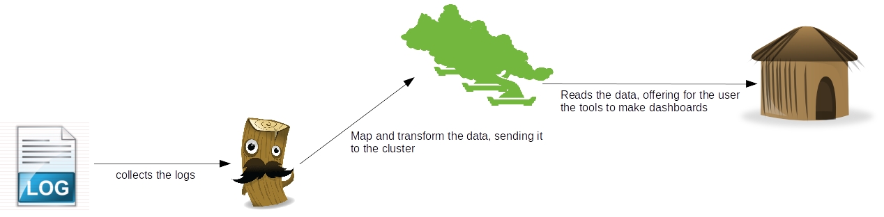
Welcome, dear reader, to another post of our series about the ELK stack for logging. On the last post, we talked about LogStash, a tool that allow us to integrate data from different sources to different destinations, using transformations along the way, in a stream-like form. On this post, we will talk about ElasticSearch, a indexer based on apache Lucene, which can allow us to organize our data and make textual searches on the data, in a scalable infrastructure. So, let’s begin by understanding how ElasticSearch is organized on the inside

Indexes, documents and shards

On ElasticSearch, we have the concept of indexes. A index is like a repository, where we can store our data in the format of documents. A document on ElasticSearch’s terminology consists of a structure for the data to be stored, analysed and classified, following a mapping definition, composed of a series of fields – a important thing to note, is that a field on ElasticSearch has the same type across the whole index, meaning that we cant have a field “phone” with the type int on a document and the type string on another.

In turn, we have our documents stored on shards, which divide the data on segments based on a rule – by default, the segmentation is made by hashing the data, but it can also be manually manipulated -, making the searches faster.

So, in a nutshell, we can say that the order of organization of ElasticSearch is as follows:

Index >> Document (mappings/type) >> shard

This organization is used by the user on the two basic operations of the cluster: indexing and searching.

One last thing to say about documents is that they can not only be stored as independent , but also be mounted on a tree-like hierarchy, with links between them. This is useful in scenarios that we can make use of hierarchical searches, such as product’s searches based on their categories.

Indexing

Indexing is the action of inputing the data from a external source to the cluster. ElasticSearch is a textual indexer, which means he can only analyse text on plain format, despite that we can use the cluster to store data in base64 format, using a plugin. Later on the post, we will see a example installation of a plugin, which are extensions we can aggregate to expand our cluster usability.

When we index our data,  we define which fields are to be analysed, which analyser to use, if the default ones does not suffice and which fields we want to store the data on the cluster, so we can use as the result of our searches. One important thing to note about the indexing operations is that, despite it has CRUD-like operations, the data is not really updated or deleted on the cluster, instead a new version is generated and the old version is marked as deleted.

This is a important thing to take note, because if not properly configured to make purges – which can be made with a configuration that break the shards into segments, and periodically make merges of the segments, phisically deleting the obsolet documents on the process -, the cluster will keep indefinitely expanding in size with the “deleted” older versions of our data, making specially the searches to became really slow.

All the operations can be made with a REST API provided by ElasticSearch, that we will see later on this post.

Searching

The other, and probably most important, action on ElasticSearch, is the searching of the data previously indexed. Like the indexing action, ElasticSearch also provide a REST API for the searches. The API provides a very rich range of possibilities of searching, from basic term searches to more complex searches such as hierarchical searches, searches by synonims, language detections, etc.

All the searching is based on a score system, where formulas are applied to confront the accuracy of the documents founded versus the query supplied. This score system can also be customized.

By default, the searching on the cluster occurs in 2 phases:

  • On the first phase, the master node sends the query for all the nodes, and subsequently shards , retrieving just the IDs and scores of the documents. Using a parameter called size which defines the maximum results from a query, the master selects the more meaningful documents, based on the score;
  • On the second phase, the master send requests for the nodes to retrieve the documents selected on the previous phase. After receiving the documents, the master finally sends the result for the client;

Alongside this search type, there’s also other modes, like the query_and_fetch. On this mode, the searching is made simultaneous on all shards, not only to retrieve the IDs and scores but also returning the data itself, limited only by the size parameter, which is applied per shard. In turn, on this mode, the maximum of results returned will be the size parameter plus the number of shards.

One interesting feature of ElasticSearch’s configuration options is the ability to make some nodes exclusive to query operations, and others to make the storage part, called data nodes. This way, when we query, our query dont need to run  across all the cluster to formulate the results, making the searches faster. On the next section we will see a little more about cluster configurations.

Cluster capabilities

When we talk about a cluster, we talk about scalability, but we also talk about availability. On ElasticSearch, we can configure the replication of shards, where the data is replicated by a given factor, so we dont lose our data if a node is lost. The replication if also maintained by the cluster, so if we lost a replica, the cluster itself will distribute a new replica for another node.

Other interesting feature of the cluster are the ability to discover itself. By the default configuration, when we start a node he will use a discovery mode called Zen, which uses unicast and multicast to search for another instances on all the ports of the OS. If it founds another instance, and the name of the cluster is the same – this is another one of the cluster’s configuration properties. All of this configurations can be made on the file elasticsearch.yml, on the config folder -, it will communicate with the instance and establish a new node for the already running cluster. There is another modes for this feature, including the discover of nodes from other servers.

Logging

The reader could be thinking: “Lol, do I need all of this to run a logging stack?”.

Of course that ElasticSearch is a very robust tool, that can be used on other solutions as well. However, on our case of making a centralized logging analysis solution, the core of ElasticSearch’s capabilities serve us well for this task, after all, we are talking about the textual analysis of log texts, for use on dashboards, reports, or simply for real-time exploration of the data.

Well, that concludes the conceptual part of our post. Now, let’s move on to the practice.

Hands-on

So, without further delay, let’s begin the hands-on. For this, we will use the previous Java program we used on our lab about LogStash. The code can be found on GitHub, on this link. On this program, we used the org.apache.log4j.net.SocketAppender from log4j to send all the logging we make to LogStash. However, on that point we just printed the messages on the console, instead of sending to ElasticSearch. Before we change this, let’s first start our cluster.

To do this, first we need to download the last version from the site and unzip the tar. Let’s open a terminal, and type the following command:

curl https://download.elasticsearch.org/elasticsearch/elasticsearch/elasticsearch-1.4.4.tar.gz | tar -zx

After running the command, we will find a new folder called “elasticsearch-1.4.4” created on the same folder we run our command. To our example, we will create 2 copies of this folder on a folder we call “elasticsearchcluster”, where each one will represent one node of the cluster. To do this, we run the following commands:

mkdir elasticsearchcluster

sudo cp -avr elasticsearch-1.4.4/ elasticsearchcluster/elasticsearch-1.4.4-node1/

sudo cp -avr elasticsearch-1.4.4/ elasticsearchcluster/elasticsearch-1.4.4-node2/

After we made our cluster structure, we dont need the original folder anymore, so we remove:

rm -R elasticsearch-1.4.4/

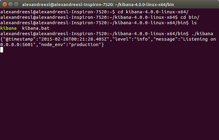
Now, let’s finally start our cluster! To do this, we open a terminal, navigate to the bin folder of our first node (elasticsearch-1.4.4-node1) and type:

./elasticsearch

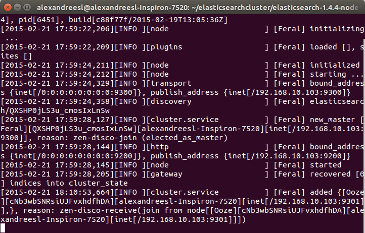
After some seconds, we can see our first node is on:

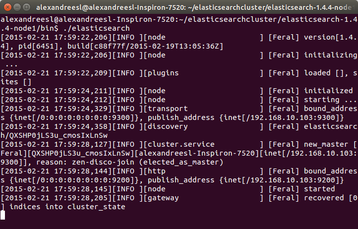
For curiosity sake, we can see the name “Feral” on the node’s name on the log. All the names generated by the tool are based on Marvel Comic’s characters. IT world sure has some sense of humor, heh?

Now, let’s start our second node. On a new terminal window, let’s navigate to the folder of our second node (elasticsearch-1.4.4-node2) and type again the command “./elasticsearch”. After some seconds, we can see that the node is also started:

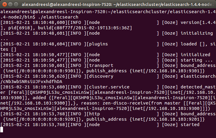
One interesting thing to notice is that our second node “Ooze”, has a mention of comunicating with our other node, “Feral”. That is the zen discover on the action, making the 2 nodes talk to each other and form a cluster. If we look again at the terminal of our first node, we can see another evidence of this bidirectional communication, as “Feral” has added “Ooze” to the cluster, as his role as a master node:

 Now that we have our cluster set up, let’s adjust our logstash script to send the messages to the cluster. To do this, let’s change the output part of the script, to the following:

input {
log4j {
port => 1500
type => “log4j”
tags => [ “technical”, “log”]
}
}

output {
stdout { codec => rubydebug }
elasticsearch_http {
host => “localhost”
port => 9200
index => “log4jlogs”
}
}

As we can see, we just included another output – we remained the console output just to check how logstash is receiving the data – including the ip and port where our ElasticSearch cluster will respond. We also defined the name of the index we want our logs to be stored. If this parameter is not defined, logstash will order elasticsearch to create a index with the pattern “logstash-%{+YYYY.MM.dd}”.

To execute this script, we do like we did on the previous post, we put the new script on a file called “configelasticsearch.conf” on the bin folder of logstash, and run with the command:

./logstash -f configelasticsearch.conf

PS1: On the GitHub repository, it is possible to find this config file, alongside a file containing all the commands we will send to ElasticSearch from now on.

PS2: For simplicity sake, we will use the default mappings logstash provide for us when sending messages to the cluster. It is also possible to pass a elasticsearch’s mapping structure, which consists of a JSON model, that logstash will use as a template. We will see the mapping from our log messages later on our lab, but for satisfying the reader curiosity for now, this is what a elasticsearch’s mapping structure look like, for example for a document type “product”:

“mappings” : {
“product”: {
“properties” : {

“variation” : { “type” : int }

“color”  : { “type” : “string” }

“code” : { “type” : int }

“quantity” : { “type” : int }

}
}
}

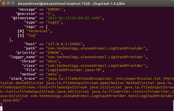
After some seconds, we can see that LogStash booted, so our configuration was a success. Now, let’s begin sending our logs!

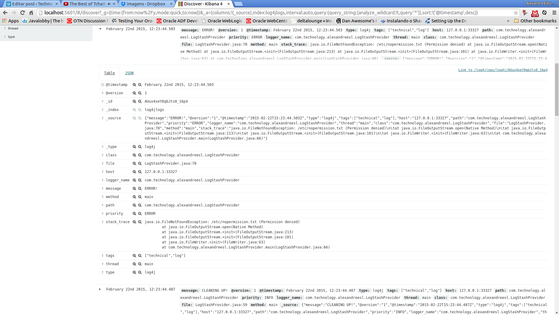
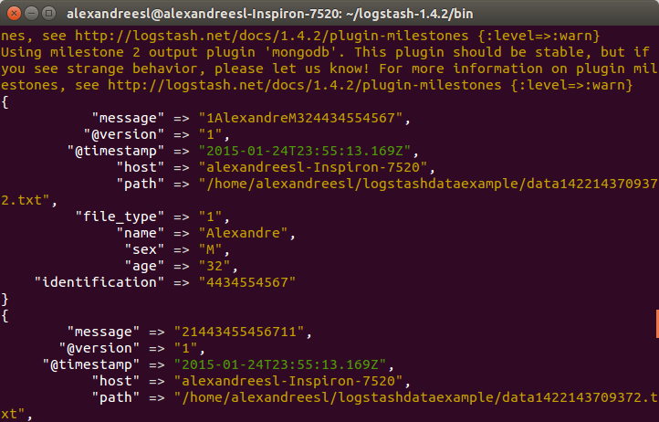
To do this, we run the program from our previous post, running the class com.technology.alexandreesl.LogStashProvider . We can see on the console of logstash, after starting the program, that the messages are going through the stack:

Now that we have our cluster up and running, let’s start to use it. First, let’s see the mappings of the index that ElasticSearch created for us, based on the configuration we made on LogStash. Let’s open a terminal and run the following command:

curl -XGET ‘localhost:9200/log4jlogs/_mapping?pretty’

On the command above, we are using ElasticSearch’s REST API. The reader will notice that, after the ip and port, the URL contains the name of the index we configured. This pattern for calls of the API is applied to most of the actions, as we can see below:

<ip>:<port>/<index>/<doc type>/<action>?<attributes>

So, after this explanation, let’s see the result from our call:

{
“log4jlogs” : {
“mappings” : {
“log4j” : {
“properties” : {
“@timestamp” : {
“type” : “date”,
“format” : “dateOptionalTime”
},
“@version” : {
“type” : “string”
},
“class” : {
“type” : “string”
},
“file” : {
“type” : “string”
},
“host” : {
“type” : “string”
},
“logger_name” : {
“type” : “string”
},
“message” : {
“type” : “string”
},
“method” : {
“type” : “string”
},
“path” : {
“type” : “string”
},
“priority” : {
“type” : “string”
},
“stack_trace” : {
“type” : “string”
},
“tags” : {
“type” : “string”
},
“thread” : {
“type” : “string”
},
“type” : {
“type” : “string”
}
}
}
}
}
}

As we can see, the index “log4jlogs” was created, alongside the document type “log4j”. Also, a series of fields were created, representing information from the log messages, like the thread that generated the log, the class, the log level and the log message itself.

Now, let’s begin to make some searches.

Let’s begin by searching all log messages which the priority was “INFO”. We make this searching by running:
curl -XGET ‘localhost:9200/log4jlogs/log4j/_search?q=priority:info&pretty=true’
A fragment of the result of the query would be something like the following:

{
“took” : 12,
“timed_out” : false,
“_shards” : {
“total” : 5,
“successful” : 5,
“failed” : 0
},
“hits” : {
“total” : 18,
“max_score” : 1.1823215,
“hits” : [ {
“_index” : “log4jlogs”,
“_type” : “log4j”,
“_id” : “AUuxkDTk8qbJts0_16ph”,
“_score” : 1.1823215,
“_source”:{“message”:”STARTING DATA COLLECTION”,”@version”:”1″,”@timestamp”:”2015-02-22T13:53:12.907Z”,”type”:”log4j”,”tags”:[“technical”,”log”],”host”:”127.0.0.1:32942″,”path”:”com.technology.alexandreesl.LogStashProvider”,”priority”:”INFO”,”logger_name”:”com.technology.alexandreesl.LogStashProvider”,”thread”:”main”,”class”:”com.technology.alexandreesl.LogStashProvider”,”file”:”LogStashProvider.java:20″,”method”:”main”}
}

.

.

.

As we can see, the result is a JSON structure, with the documents that met our search. The beginning information of the result is not the documents themselves, but instead information about the search itself, such as the number of shards used, the seconds the search took to execute, etc. This kind of information is useful when we need to make a tuning of our searches, like manually defining the shards we which to use on the search, for example.

Let’s see another example. On our previous search, we received all the fields from the document on the result, which is not always the desired result, since we will not always use the whole information. To limit the fields we want to receive, we make our query like the following:
curl -XGET ‘localhost:9200/log4jlogs/log4j/_search?pretty=true’ -d ‘
{
“fields” : [ “priority”, “message”,”class” ],
“query” : {
“query_string” : { “query” : “priority:info” }
}
}’
On the query above, we asked ElasticSearch to limit the return to only return the priority, message and class fields. A fragment of the result can be seen bellow:

.

.

.

{
“_index” : “log4jlogs”,
“_type” : “log4j”,
“_id” : “AUuxkECZ8qbJts0_16pr”,
“_score” : 1.1823215,
“fields” : {
“priority” : [ “INFO” ],
“message” : [ “CLEANING UP!” ],
“class” : [ “com.technology.alexandreesl.LogStashProvider” ]
}
}

.

.

.

Now, let’s use the term search. On the term searches, we use ElasticSearch’s textual analysis to find a term inside the text of a field. Let’s run the following command:
curl -XGET ‘localhost:9200/log4jlogs/log4j/_search?pretty=true’ -d ‘
{
“fields” : [ “priority”, “message”,”class” ],
“query” : {
“term” : {
“message” : “up”
}
}
}’
If we see the result, it would be all the log messages that contains the word “up”. A fragment of the result can be seen bellow:

{
“_index” : “log4jlogs”,
“_type” : “log4j”,
“_id” : “AUuxkESc8qbJts0_16pv”,
“_score” : 1.1545612,
“fields” : {
“priority” : [ “INFO” ],
“message” : [ “CLEANING UP!” ],
“class” : [ “com.technology.alexandreesl.LogStashProvider” ]
}
}

Of course, there is a lot more of searching options on ElasticSearch, but the examples provided on this post are enough to make a good starting point for the reader. To make a final example, we will use the “prefix” search. On this type of search, ElasticSearch will search for terms that start with our given text, on a given field. For example, to search for log messages that have words starting with “clea”, part of the word “cleaning”, we run the following:
curl -XGET ‘localhost:9200/log4jlogs/log4j/_search?pretty=true’ -d ‘
{
“fields” : [ “priority”, “message”,”class” ],
“query” : {
“prefix” : {
“message” : “clea”
}
}
}’
If we see the results, we will see that are the same from the previous search, proving that our search worked correctly.

Kopf

The reader possibly could ask “Is there another way to send my queries without using the terminal?” or “Is there any graphical tool that I can use to monitor the status of my cluster?”. As a matter of fact, there is a answer for both of this questions, and the answer is the kopf plugin.

As we said before, plugins are extensions that we can install to improve the capacities of our cluster. In order to install the plugin, first let’s stop both the nodes of the cluster – press ctrl+c on both terminal windows to stop – then, navigate to the nodes root folder and type the following:

bin/plugin -install lmenezes/elasticsearch-kopf

If the plugin was installed correctly, we should see a message like the one bellow on the console:

.

.

.

-> Installing lmenezes/elasticsearch-kopf…
Trying https://github.com/lmenezes/elasticsearch-kopf/archive/master.zip&#8230;
Downloading …………………………………………………………………………………………………………………………………………………………………………………………………………………………………………………………………………………………………………………………………………………………………………………………………………………………………………………………………………………………………………………………………..DONE
Installed lmenezes/elasticsearch-kopf into….

After installing on both nodes, we can start again the nodes, just as we did before. After the booting of the cluster, let’s open a browser and type the following URL:

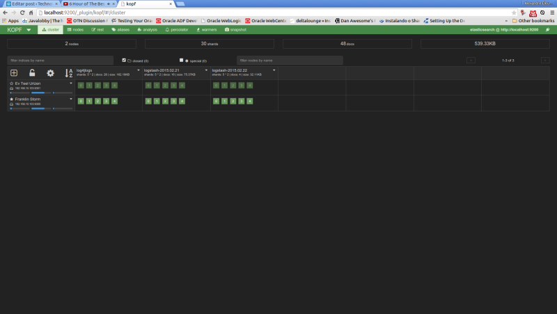
http://localhost:9200/_plugin/kopf

We will see the following web page of the kopf plugin, showing the status of our cluster, such as the nodes, the indexes, shard information, etc

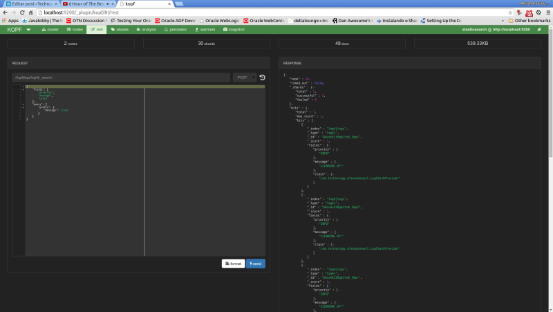
Now, let’s run our last example from the search queries on kopf. First, we select the “rest” option on the top menu. On the next screen, we select “POST” as the http method, include on the URL field the index and document type to narrow the results and on the textarea bellow we include our JSON query filters. The print bellow shows the query made on the interface:

 Conclusion

And so we conclude our post about ElasticSearch. A very powerful tool on the indexing and analysis of textual information, the central stone on our ELK stack for logging is a tool to be used, not only on a logging analysis system, but on other solutions that his features can be useful as well.

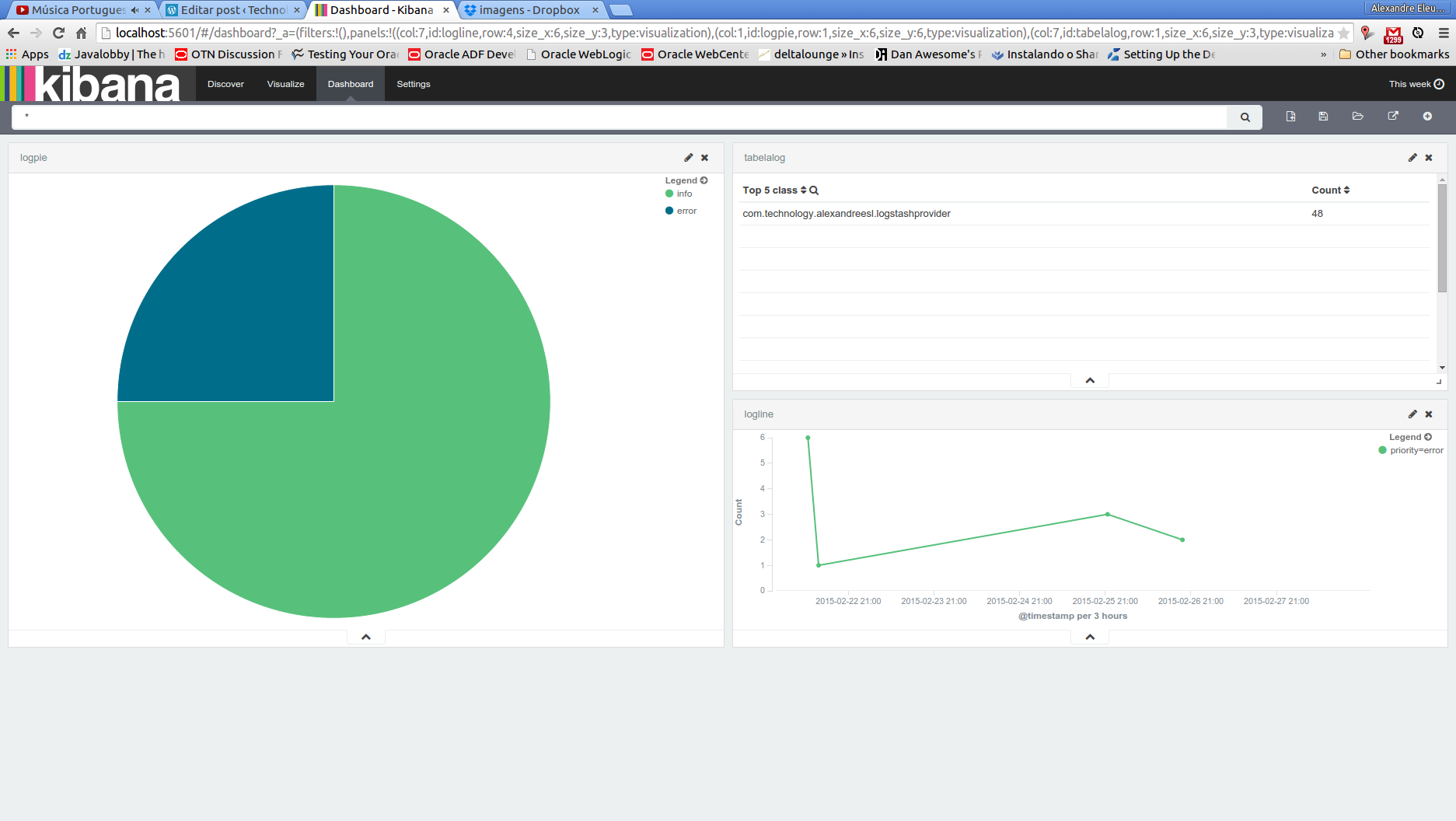
So, our stack is almost complete. We can gather our log information, and the information is indexed on our cluster. However, a final piece remains: we need a place where we can have a more friendly interface, that allow us not only to search the information, but also to make rich presentations of the data, such as dashboards. That’s when it enters our last part of our ELK series and the last tool we will see, Kibana. Thank you for following me on another post, until next time.

Continue reading

ELK: using a centralized logging architecture – part 1

Standard

Welcome, dear reader, to another post from my blog. On this new series, we will talk about a architecture specially designed to process data from log files coming from applications, with the junction of 3 tools, Logstash, ElasticSearch and Kibana. But after all, do we really need such a structure to process log files?

Stacks of log

On a company ecosystem, there is lots of systems, like the CRM, ERP, etc. On such environments, it is common for the systems to produce tons of logs, which provide not only a real-time analysis of the technical status of the software, but could also provide some business information too, like a log of a customer’s behavior  on a  shopping cart, for example. To dive into this useful source of information, enters the ELK architecture, which name came from the initials of the software involved: ElasticSearch, LogStash and Kibana. The picture below shows in a macro vision the flow between the tools:

As we can see, there’s a clear separation of concerns between the tools, where which one has his own individual part on the processing of the log data:

  • Logstash: Responsible for collect the data, make transformations like parsing – using regular expressions – adding fields, formatting as structures like JSON, etc and finally sending the data to various destinations, like a ElasticSearch cluster. Later on this post we will see more detail about this useful tool;
  •  ElasticSearch: RESTful data indexer, ElasticSearch provides a clustered solution to make searches and analysis on a set of data. On the second part of our series, we will see more about this tool;
  • Kibana: Web-based application, responsible for providing a light and easy-to-use dashboard tool. On the third and last part of our series, we will see more of this tool;

So, to begin our road in the ELK stack, let’s begin by talking about the tool responsible for integrating our data: LogStash.

LogStash installation

To install, all we need to do is unzip the file we get from LogStash’s site and run the binaries on the bin folder. The only pre-requisite for the tool is to have Java installed and configured in the environment. If the reader wants to follow my instructions with the same system then me, I am using Ubuntu 14.10 with Java 8, which can be downloaded from Oracle’s site here.

With Java installed and configured, we begin by downloading and unziping the file. To do this, we open a terminal and input:

curl https://download.elasticsearch.org/logstash/logstash/logstash-1.4.2.tar.gz | tar xz

After the download, we will have LogStash on a folder on the same place we run our ‘curl’ command. On the LogStash terminology, we have 4 types of configurations we can make for a stream, named:

  • input: On this configuration, we put the sources of our streams, that can range from polling files of a file system to more complex inputs such as a Amazon SQS queue and even Twitter;
  • codec: On this configuration we make transformations on the data, like turning into a JSON structure, or grouping together lines that are semantically related, like for example, a Java’s stack trace;
  • filter: On this configuration we make operations such as parsing data from/to different formats, removal of special characters and checksums for deduplication;
  • output: On this configuration we define the destinations for the processed data, such as a ElasticSearch cluster, AWS SQS, Nagios etc;

Now that we have established LogStash’s configuration structure, let’s begin with our first execution. In LogStash we have two ways to configure our execution, one way by providing the settings on the start command itself and the other one is by providing a configuration file for the command. The simplest way to boot a LogStash’s stream is by setting the input and output as the console itself, to make this execution, we open a terminal, navigate to the bin folder of our LogStash’s installation and execute the following command:

./logstash -e ‘input { stdin { } } output { stdout {} }’

As we can see after we run the command, we booted LogStash, setting the console as the input and the output, without any transformation or filtering. To test, we simply input anything on the console, seeing that our message is displayed back by the tool:

Now that we get the installation out of the way, let’s begin with the actual lab. Unfortunately -or not, depending on the point of view -, it would take us a lot of time to show all the features of what we can do with the tool, so to make a short but illustrative example, we will start 2 logstash streams, to do the following:

1st stream:

  • The input will be made by a java program, which will produce a log file with log4j, representing technical information;
  • For now, we will just print logstash’s events on the console, using the rubydebug codec. On our next part on the series, we will return to this configuration and change the output to send the events to elasticsearch;

2nd stream:

  • The input will be made by the same java program, which will produce a positional file, representing business information of costumers and orders;
  • We will then use the grok filter to parse the data of the positional file into separated fields, producing the data for the output step;
  • Finally, we use the mongodb output, to save our data – filtering to only persist the orders – on a  Mongodb collection;

With the streams defined, we can begin our coding. First, let’s create the java program which will generate the inputs for the streams. The code for the program can be seen bellow:

package com.technology.alexandreesl;

import java.io.FileWriter;
import java.io.IOException;
import java.io.PrintWriter;
import java.util.ArrayList;
import java.util.Date;
import java.util.List;

import org.apache.log4j.Logger;

public class LogStashProvider {

private static Logger logger = Logger.getLogger(LogStashProvider.class);

public static void main(String[] args) throws IOException {

try {

logger.info(“STARTING DATA COLLECTION”);

List<String> data = new ArrayList<String>();

Customer customer = new Customer();
customer.setName(“Alexandre”);
customer.setAge(32);
customer.setSex(‘M’);
customer.setIdentification(“4434554567”);

List<Order> orders = new ArrayList<Order>();

for (int counter = 1; counter < 10; counter++) {

Order order = new Order();

order.setOrderId(counter);
order.setProductId(counter);
order.setCustomerId(customer.getIdentification());
order.setQuantity(counter);

orders.add(order);

}

logger.info(“FETCHING RESULTS INTO DESTINATION”);

PrintWriter file = new PrintWriter(new FileWriter(
“/home/alexandreesl/logstashdataexample/data”
+ new Date().getTime() + “.txt”));

file.println(“1” + customer.getName() + customer.getSex()
+ customer.getAge() + customer.getIdentification());

for (Order order : orders) {
file.println(“2” + order.getOrderId() + order.getCustomerId()
+ order.getProductId() + order.getQuantity());
}

logger.info(“CLEANING UP!”);

file.flush();
file.close();

// forcing a error to simulate stack traces
PrintWriter fileError = new PrintWriter(new FileWriter(
“/etc/nopermission.txt”));

} catch (Exception e) {

logger.error(“ERROR!”, e);
}

}

}

As we can see, it is a very simple class, that uses log4j to generate some log and output a positional file representing data from customers and orders and at the end, try to create a file on a folder we don’t have permission to write by default, “forcing” a error to produce a stack trace. The complete code for the program can be found here. Now that we have made our data generator, let’s begin the configuration for logstash. The configuration for our first example is the following:

input {
log4j {
port => 1500
type => “log4j”
tags => [ “technical”, “log”]
}
}

output {
stdout { codec => rubydebug }
}

To run the script, let’s create a file called “config1.conf” and save the file with the script on the “bin” folder of logstash’s installation folder. Finally, we run the script with the following command:

 ./logstash -f config1.conf

This will start logstash process with the configurations we provided. To test, simply run the java program we coded earlier and we will see a sequence of message events in logstash’s console window, generated by the rubydebug codec, like the one bellow, for example:

{
“message” => “ERROR!”,
“@version” => “1”,
“@timestamp” => “2015-01-24T19:08:10.872Z”,
“type” => “log4j”,
“tags” => [
[0] “technical”,
[1] “log”
],
“host” => “127.0.0.1:34412”,
“path” => “com.technology.alexandreesl.LogStashProvider”,
“priority” => “ERROR”,
“logger_name” => “com.technology.alexandreesl.LogStashProvider”,
“thread” => “main”,
“class” => “com.technology.alexandreesl.LogStashProvider”,
“file” => “LogStashProvider.java:70”,
“method” => “main”,
“stack_trace” => “java.io.FileNotFoundException: /etc/nopermission.txt (Permission denied)\n\tat java.io.FileOutputStream.open(Native Method)\n\tat java.io.FileOutputStream.<init>(FileOutputStream.java:213)\n\tat java.io.FileOutputStream.<init>(FileOutputStream.java:101)\n\tat java.io.FileWriter.<init>(FileWriter.java:63)\n\tat com.technology.alexandreesl.LogStashProvider.main(LogStashProvider.java:66)”
}

Now, let’s move on to the next stream. First, we create another file, called “config2.conf”, on the same folder we created the first one. On this new file, we create the following configuration:

input {
file {
path => “/home/alexandreesl/logstashdataexample/data*.txt”
start_position => “beginning”
}
}

filter {
grok {
match => [ “message” , “(?<file_type>.{1})(?<name>.{9})(?<sex>.{1})(?<age>.{2})(?<identification>.{10})” , “message” , “(?<file_type>.{1})(?<order_id>.{1})(?<costumer_id>.{10})(?<product_id>.{1})(?<quantity>.{1})” ]
}
}

output {
stdout { codec => rubydebug }
if [file_type] == “2” {
mongodb {
collection => “testData”
database => “mydb”
uri => “mongodb://localhost”
}
}
}

With the configuration created, we can run our second example. Before we do that, however, let’s dive a little on the configuration we just made. First, we used the file input, which will make logstash keep monitoring the files on the folder and processing them as they appear on the input folder.

Next, we create a filter with the grok plugin. This filter uses combinations of regular expressions, that parses the data from the input. The plugin comes with more then 100 patterns pre-made that helps the development. Another useful tool in the use of grok is a site where we could test our expressions before use. Both links are available on the links section at the end of this post.

Finally, we use the mongodb plugin, where we reference our logstash for a database and collection of a mongodb instance, where we will insert the data from the file into mongodb’s documents. We also used again the rubydebug codec, so we can also see the processing of the files on the console. The reader will note that we used a “if” statement before the configuration of the mongodb output. After we parse the data with grok, we can use the newly created fields to do some logic on our stream. In this case, we filter to only process data with the type “2”, so only the order’s data goes to the collection on mongodb, instead of all the data. We could have expanded more on this example, like saving the data into two different collections, but for the idea of passing a general view of the structure of logstash for the reader, the present logic will suffice.

PS: This example assumes the reader has mongodb installed and running on the default port of his environment, with a db “mydb” and a collection “testData” created. If the reader doesn’t have mongodb, the instructions can be found on the official documentation.

Finally, with everything installed and configured, we run the script, with the following command:

./logstash -f config2.conf

After logstash’s start, if we run our program to generate a file, we will see logstash working the data, like the screen bellow:

And finally, if we query the collection on mongodb, we see the data is persisted:

Conclusion

And so we conclude the first part of our series. With a simple usage, logstash prove to be a useful tool in the integration of information from different formats and sources, specially log-related. In the next part of our series, we will dive in the next tool of our stack: ElasticSearch. Until next time

Continue reading