gRPC: Transporting massive data with Google’s serialization

Hello, dear readers! Welcome to my blog. On this post, we will delve on Google’s RPC style solution, gRPC and his serialization technique, protocol buffers. But what is gRPC and why it is so useful? Let’s find out!

The escalation of data transfer

When developing APIs, one of the most common ways of implementing the interface is with REST, using HTTP and JSON as transportation protocol and data schema, respectively. At first, there is no problem with this approach, and most of the time we won’t need to change from this kind of stack.

However, the problems begin when we get a API that has a big continuous volume of requests. On a situation like this, the amount of memory used on tasks like data transportation could begin to be a burden on the API, making calls more and more slow.

It is on this scenario that gRPC comes in handy. With a server-client model and a serialization technique from Google’s that allows us to shrink the amount of resources used on remote calls, we can scale more capacity per API instance, making our APIs more powerful.

This comes with a price, however: operations like debugging get more difficult on this scenario, because gRPC encapsulates the transportation logic on Google’s solution that utilizes binary serialization to do the transportation, so it is not as easily debuggable as a common plain REST/JSON application.

RPC

RPC is a acronym for Remote Procedure Call, a old model that was much used on the past. On that model, a client-server solution is developed, where the details of transport are abstracted from the developer, been responsible only for implementing the server and client inner logic. Famous RPC models were CORBA, RMI and DCOM.

Despite the name, gRPC only has the concept of a client-server application in common with the old solutions, that suffered from problems such as incompatible protocols between each other, alongside with not offering more advanced techniques from today, such as streams. Their solutions reminds more of the classical request-response model, from the first days of the web.

gRPC

So what is gRPC? This is Google’s approach to a client-server application that takes principles from the original RPC. However, gRPC allows us to use more sophisticated technologies such as HTTP2 and streams. gRPC is also designed as technology-agnostic, which means that can be used and interacted with server and clients from different programming languages.

With gRPC we develop gRPC services, which are generated based on a proto file we provide. Using the proto file, gRPC generates for us a server and a stub (some languages just call it a client) where we develop our server and client logic. The following diagram, taken from gRPC documentation, represents the client-server schematics:

As we can see on the diagram, gRPC supplies us with different types of languages to choose from to develop /expose our gRPC services. At the time of this post, gRPC supports Java, C++, Python, Objective-C, C#, a lite-runtime (Android Java), Ruby, JavaScript and Go – using the golang/protobuf library.

Protocol Buffers

Protocol buffer is gRPC’s serialization mechanism, which allows us to send compressed messages between our services, allowing us in turn to process more data with less network roundtrips between the parts.

According to Protocol Buffers documentation, Protocol Buffers messages offers the following advantages, if we compare to a traditional data schema such as XML:

are simpler
are 3 to 10 times smaller
are 20 to 100 times faster
are less ambiguous
generate data access classes that are easier to use programmatically

The Protocol Buffers framework supplies us with several code generators for different programming languages. If we want to develop on Java, for instance, we download Protocol Buffers for Java, then we model a proto file where we design the schema for the messages we will transport and then we generate code using the protoc compiler.

The compiler will generate code for us in order to use for serialize/deserialize data on the format we provided on the proto file.

Types of gRPC applications

gRPC applications can be written using 3 types of processing, as follows:

Unary RPCs: The simplest type and more close to classical RPC, consists of a client sending one message to a server, that makes some processing and returns one message as response;
Server streams: On this type, the client sends one message for the server, but receives a stream of messages from the server. The client keeps reading the messages from the server until there is no more messages to read;
Client streams: This type is the opposite of the server streams one, where on this case is the client who sends a stream of messages to make a request for the server and them waits for the server to produce a single response for the series of request messages provided;
Bidirecional stream RPC: This is the more complex but also more dynamic of all the types. On this model, we have both client and server reading and writing on streams, which are stablished between the server and client. This streams are independent from each other, which means that could be possible for a client to send a message to a server by one stream and vice-versa at the same time. This allows us to make multiple processing scenarios, such as clients sending all the messages before the responses, clients and servers “ping-poinging” messages between each other and so on.

Synch vs. Asynch

As the name implies, synchronous processing occurs when we have a communication where the client thread is blocked when a message is sent and is been processed.

Asynchronous processing occurs when we have this communication with the processing been done by other threads, making the whole process been non-blocking.

On gRPC we have both styles of processing supported, so it is up to the developer to use the better approach for his solutions.

Deadlines & timeouts

A deadline stipulates how much time a gRPC client will wait on a RPC call to return before assuming a problem has happened. On the server’s side, the gRPC services can query this time, verifying how much time it has left.

If a response couldn’t be received before the deadline is met, a DEADLINE_EXCEEDED error is thrown and the RPC call is terminated.

RPC termination

On gRPC, both clients and servers decide if a RPC call is finished or not locally and independently. This means that a server can decide to end a call before a client has transmitted all their messages and a client can decide to end a call before a server has transmitted one or all of their responses.

This point is important to remember specially when working with streams, in a sense that logic must pay attention to possible RPC terminations when treating sequences of messages.

Channels

Channels are the way a client stub can connect with gRPC services on a given host and port. Channels can be configured specific by client, such as turning message compression on and off for a specific client.

Tutorial

On this lab we will implement a gRPC service, test by making some calls and experimenting a little with streams. It will get us a feel and a head start on how to develop solutions using gRPC.

Set up

For this lab we will use Python 3.4. For the coding, I like to use Pycharm, is a really good IDE for Python that the reader can find it here.

For containerization I used Docker 17.03.1-ce. I also recommend you create a virtual environment for the lab, using virtualenv.

Let’s create a new virtual environment for our lab. On a terminal, let’s type the following:

virtualenv --python=python3.4 -v grpc-handson

After running the command, we will see that a folder was created. That is our virtual environment.

To install gRPC, first we enable the virtual environment on our terminal session. we do this by typing the following, assuming we are inside the virtual environment’s folder:

source ./bin/activate

This will change our terminal, that will now show a prefix with our env’s name, showing it is enabled.

Now on to the installation. First, let’s install gRPC with pip by typing:

python -m pip install grpcio

We also need to install gRPC tools. This tools are responsible for installing the protoc compiler which we will use later on the lab. We install it by typing:

python -m pip install grpcio-tools

That’s it! Now that we have our environment, let’s start with the development.

Creating the gRPC Service definition

First, we create a gRPC Service definition. We create this by coding a proto file, which will have the following:

syntax = "proto3";

option java_multiple_files = true;
option java_package = "com.alexandreesl.handson";
option java_outer_classname = "MyServiceProto";
option objc_class_prefix = "HLW";

package handson;


service MyService {

    rpc MyMethod1 (MyRequest) returns (MyResponse) {
    }

    rpc MyMethod2 (MyRequest) returns (MyResponse) {
    }

}

message MyRequest {
    string name = 1;
    int32 code = 2;
}

message MyResponse {
    string name = 1;
    string sex = 2;
    int32 code = 3;
}

This file is based on examples from the official gRPC repo – you can find the link at the end of this post. Alongside setting some properties such as the service’s package, we defined a service with 2 methods and 2 schemas for the protocol buffers, used by the methods.

With the proto file created (let’s save it as my_service.proto), it is time for us to use gRPC to create the code.

Generating gRPC code

To generate the code, let’s run the following command, with our virtual environment enabled and on the same folder of the proto file:

 python -m grpc_tools.protoc -I. --python_out=. --grpc_python_out=. my_service.proto

After running the command, we will see 2 files created, as we can see bellow:

PS: The source code for our lab can be found at the end of the post.

Building the server

Now that we have our code generated, let’s begin our work. Let’s begin by creating the server side.

The code from our command is auto-generated, so is not a good practice to code on them. Instead, for the server we will extend the servicer class, so we implement our own gRPC service without editing generated code.

Let’s create a file called gRPC_server.py and add the following code:

import time
from concurrent import futures

import grpc

import my_service_pb2 as my_service_pb2
import my_service_pb2_grpc as my_service_pb2_grpc

_ONE_DAY_IN_SECONDS = 60 * 60 * 24


class gRPCServer(my_service_pb2_grpc.MyServiceServicer):
    def __init__(self):
        print('initialization')

    def MyMethod1(self, request, context):
        print(request.name)
        print(request.code)
        return my_service_pb2.MyResponse(name=request.name, sex='M', code=123)

    def MyMethod2(self, request, context):
        print(request.name)
        print(request.code * 12)
        return my_service_pb2.MyResponse(name=request.name, sex='F', code=1234)


def serve():
    server = grpc.server(futures.ThreadPoolExecutor(max_workers=10))
    my_service_pb2_grpc.add_MyServiceServicer_to_server(
        gRPCServer(), server)
    server.add_insecure_port('[::]:50051')
    server.start()
    try:
        while True:
            time.sleep(_ONE_DAY_IN_SECONDS)
    except KeyboardInterrupt:
        server.stop(0)


if __name__ == '__main__':
    serve()

On the code above we created a class that it is a subclass of the class generated by the protoc compiler. We can see that in order to get the request’s parameters, all we have to do is navigate from the request object. To generate a response, all we have to do is instantiate the appropriate class.

We also coded the serve method, where we created a server with 10 worker threads to serve requests and initialized with the class we created to implement the server-side.

To start the server, all we have to do is run:

python gRPC_server.py

And from now on, unless we kill the process, it will be answering on the 50051 port.

Now that we created the server, let’s begin the work on the client.

Constructing the client

In order to consume the server, we need to create a client for our stub. Let’s do this.

Let’s create a file called gRPC_client.py and code the following:

import grpc

import my_service_pb2 as my_service_pb2
import my_service_pb2_grpc as my_service_pb2_grpc


class gRPCClient():
    def __init__(self):
        channel = grpc.insecure_channel('localhost:50051')
        self.stub = my_service_pb2_grpc.MyServiceStub(channel)

    def method1(self, name, code):
        print('method 1')
        return self.stub.MyMethod1(my_service_pb2.MyRequest(name=name, code=code))

    def method2(self, name, code):
        print('method 2')
        return self.stub.MyMethod2(my_service_pb2.MyRequest(name=name, code=code))


def main():
    print('main')

    client = gRPCClient()

    print(client.method1('Alexandre', 123))
    print(client.method2('Maria', 123))


if __name__ == '__main__':
    main()

As we can see, is really simple to create a client: we just needed to establish a channel and instantiate a stub with it. Once instantiated, we just need to call the methods on the stub as we normally would do with any Pythonic object.

Now that we have the coding done, let’s test some calls!

Making the call

To test a call, let’s first start the server. With a terminal session opened and our virtual environment enabled, let’s start the server, by entering the command we talked about earlier:

python gRPC_server.py

And on another terminal, started like the previous one, we call the client by typing:

python gRPC_client.py

After firing up the client, we will see that the client produced the following output:

main
method 1
name: "Alexandre"
sex: "M"
code: 123

method 2
name: "Maria"
sex: "F"
code: 1234

And on the server terminal, we can see the following output:

initialization
Alexandre
123
Maria
1476

Success! We have implemented our first gRPC service. Now, let’s wrap it up our lab by seeing the last topics: using streams and containerization.

Using streams

To learn about streams, let’s add a new method, that it will be a bidirectional streaming.

First, let’s change the proto file, creating a new method, like the following:

syntax = "proto3";

option java_multiple_files = true;
option java_package = "com.alexandreesl.handson";
option java_outer_classname = "MyServiceProto";
option objc_class_prefix = "HLW";

package handson;


service MyService {

    rpc MyMethod1 (MyRequest) returns (MyResponse) {
    }

    rpc MyMethod2 (MyRequest) returns (MyResponse) {
    }

    rpc MyMethod3 (stream MyRequest) returns (stream MyResponse) {
    }

}

message MyRequest {
    string name = 1;
    int32 code = 2;
}

message MyResponse {
    string name = 1;
    string sex = 2;
    int32 code = 3;
}

That’s right, this is everything we need to do. After generating the files from the proto again, we need to modify our server to reflect the changes. We do this modifying the file as follows:

import time
from concurrent import futures

import grpc

import my_service_pb2 as my_service_pb2
import my_service_pb2_grpc as my_service_pb2_grpc

_ONE_DAY_IN_SECONDS = 60 * 60 * 24


class gRPCServer(my_service_pb2_grpc.MyServiceServicer):
    def __init__(self):
        print('initialization')

    def MyMethod1(self, request, context):
        print(request.name)
        print(request.code)
        return my_service_pb2.MyResponse(name=request.name, sex='M', code=123)

    def MyMethod2(self, request, context):
        print(request.name)
        print(request.code * 12)
        return my_service_pb2.MyResponse(name=request.name, sex='F', code=1234)

    def MyMethod3(self, request_iterator, context):
        for req in request_iterator:
            print(req.name)
            print(req.code)

            yield my_service_pb2.MyResponse(name=req.name, sex='M', code=123)


def serve():
    server = grpc.server(futures.ThreadPoolExecutor(max_workers=10))
    my_service_pb2_grpc.add_MyServiceServicer_to_server(
        gRPCServer(), server)
    server.add_insecure_port('[::]:50051')
    server.start()
    try:
        while True:
            time.sleep(_ONE_DAY_IN_SECONDS)
    except KeyboardInterrupt:
        server.stop(0)


if __name__ == '__main__':
    serve()

As we can see, the new MyMethod3 receives a iterator of request messages and also send a series of responses as well, by using the yield keyword, which teaches Python to create a generator from our function. We can read more about the yield keyword on this link.

Now we modify the client. We also use a generator with the yield keyword, but on this case, we make the generator create each item at random time intervals, to simulate a real life application with data entering at intervals. The response stream is read with a simple for loop, that it will continue to run until there is no data to output:

import random
import time

import grpc

import my_service_pb2 as my_service_pb2
import my_service_pb2_grpc as my_service_pb2_grpc


class gRPCClient():
    def __init__(self):
        channel = grpc.insecure_channel('localhost:50051')
        self.stub = my_service_pb2_grpc.MyServiceStub(channel)

    def method1(self, name, code):
        print('method 1')
        return self.stub.MyMethod1(my_service_pb2.MyRequest(name=name, code=code))

    def method2(self, name, code):
        print('method 2')
        return self.stub.MyMethod2(my_service_pb2.MyRequest(name=name, code=code))

    def method3(self, req):
        print('method 3')
        return self.stub.MyMethod3(req)


def generateRequests():
    reqs = [my_service_pb2.MyRequest(name='Alexandre', code=123), my_service_pb2.MyRequest(name='Maria', code=123),
            my_service_pb2.MyRequest(name='Eleuterio', code=123), my_service_pb2.MyRequest(name='Lucebiane', code=123),
            my_service_pb2.MyRequest(name='Ana Carolina', code=123)]

    for req in reqs:
        yield req
        time.sleep(random.uniform(2, 4))


def main():
    print('main')

    client = gRPCClient()

    print(client.method1('Alexandre', 123))
    print(client.method2('Maria', 123))

    res = client.method3(generateRequests())

    for re in res:
        print(re)


if __name__ == '__main__':
    main()

If we restart the server and run the new client, we will receive the following output:

main
method 1
name: "Alexandre"
sex: "M"
code: 123

method 2
name: "Maria"
sex: "F"
code: 1234

method 3
name: "Alexandre"
sex: "M"
code: 123

name: "Maria"
sex: "M"
code: 123

name: "Eleuterio"
sex: "M"
code: 123

name: "Lucebiane"
sex: "M"
code: 123

name: "Ana Carolina"
sex: "M"
code: 123


Process finished with exit code 0

Please note that all this calls were made using the synchronous approach, so the client thread is locked each time a call is made. If we wanted to call the server asynchronously, we would use Python’s futures to do so. I suggest the reader to explore this option as a post-lab exercise.

Running gRPC on Docker

Finally, we would want to run our gRPC server on a Docker container. That is a very simple task to do.

First, let’s create a Dockerfile like the following:

FROM grpc/python:1.0-onbuild
CMD [ "python", "./gRPC_server.py" ]

Yup, that’s all! This is a official image from gRPC which makes a pip install on a requirements file and adds the current directory on the container, so we don’t need to add the files ourselves. Let’s build the container:

docker build -t alexandreesl/grpc-lab .

And finally, launch it with our image:

docker run --rm -p 50051:50051 alexandreesl/grpc-lab

If we run again the client, we will see that the server was successfully started. If the reader want, you can also start the container directly by a image I created on Docker Hub for this lab, already built with the source code from our lab. To pull the image, just type the following:

docker pull alexandreesl/grpc-lab

Conclusion

And so we concludes another journey on our great world of technology. I hope I could help the reader to understand what is gRPC and how it can be used to improve our capacity on high demanding API scenarios. Thank you for following me on this post, see you next time.

Curator: Implementing purge routines on your Elasticsearch cluster

Hi, dear readers! Welcome to my blog. On this post, we will learn how to use the Curator project to create purge routines on a Elasticsearch cluster.

When we have a cluster crunching logs and other data types from our systems, it is necessary to configure process that manages this data, doing actions like purges and backups. For this purpose, the Curator project comes in handy.

Curator is a Python tool, that allows several types of actions. On this post, we will focus on 2 actions, purge and backup. To install Curator, we can use pip, like the command bellow:

sudo pip install elasticsearch-curator

Once installed, let’s begin preparing our cluster to make the backups, by a backup repository. A backup repository is a Elasticsearch feature, that process backups and save them on a persistent store. On this case, we will configure the backups to be stored on a Amazon S3 bucket. First, let’s install AWS Cloud plugin for Elasticsearch, by running the following command on each of the cluster’s nodes:

bin/plugin install cloud-aws

And before we restart our nodes, we configure the AWS credentials for the cluster to connect to AWS, by configuring them on the elasticsearch.yml file:

cloud:
  aws:
    access_key: <access key>
    secret_key: <secret key>

Finally, let’s configure our backup repository, using Elasticsearch REST API:

PUT /_snapshot/elasticsearch_backups
{
 “type”: “s3”,
 “settings”: {
 “bucket”: “elastic-bckup”,
 “region”: “us-east-1”
 }
}

On the command above, we created a new backup repository, called “elasticsearch-backups”, also defining the bucket where the backups will be created. With our repository created, let’s create our YAMLs to configure Curator.

The first YAML is “curator-config.yml”, where we configure details such as the cluster address. A configuration example could be as follows:

client:
  hosts:
    — localhost
  port: 9200
  url_prefix:
  use_ssl: False
  certificate:
  client_cert:
  client_key:
  aws_key:
  aws_secret_key:
  aws_region:
  ssl_no_validate: False
  http_auth:
  timeout: 240
  master_only: False
logging:
  loglevel: INFO
  logfile:
  logformat: default
  blacklist: [‘elasticsearch’, ‘urllib3’]

The other YAML is “curator-action.yml”, where we configure a action list to be executed by Curator. On the example, we have indexes of data from Twitter, with the prefix “twitter”, where we first create a backup from indexes that are more then 2 days old and after the backup, we purge the data:

actions:
 1:
   action: snapshot
   description: >-
     Make backups of indices older then 2 days.
   options:
     repository: elasticsearch_backups
     name: twitter-%Y.%m.%d
     ignore_unavailable: False
     include_global_state: True
     partial: False
     wait_for_completion: True
     skip_repo_fs_check: False
     timeout_override:
     continue_if_exception: False
     disable_action: False
   filters:
   — filtertype: age
     source: creation_date
     direction: older
     unit: days
     unit_count: 2
     exclude:
  2:
    action: delete_indices
    description: >-
      Delete indices older than 2 days (based on index name).
    options:
      ignore_empty_list: True
      timeout_override:
      continue_if_exception: False
      disable_action: False
    filters:
    — filtertype: pattern
      kind: prefix
      value: twitter-
      exclude:
    — filtertype: age
      source: name
      direction: older
      timestring: ‘%Y.%m.%d’
      unit: days
      unit_count: 2
      exclude:

With the YAMLs configured, we can execute Curator, with the following command:

curator — config curator-config.yml curator-action.yml

The command will generate a log from the actions performed, showing that our configurations were a success:

2016–08–27 16:14:36,576 INFO Action #1: snapshot
2016–08–27 16:14:40,814 INFO Creating snapshot “twitter-2016.08.27” from indices: [u’twitter-2016.08.14', u’twitter-2016.08.25']
2016–08–27 16:15:34,725 INFO Snapshot twitter-2016.08.27 successfully completed.
2016–08–27 16:15:34,725 INFO Action #1: completed
2016–08–27 16:15:34,725 INFO Action #2: delete_indices
2016–08–27 16:15:34,769 INFO Deleting selected indices: [u’twitter-2016.08.14', u’twitter-2016.08.25']
2016–08–27 16:15:34,769 INFO — -deleting index twitter-2016.08.14
2016–08–27 16:15:34,769 INFO — -deleting index twitter-2016.08.25
2016–08–27 16:15:34,860 INFO Action #2: completed
2016–08–27 16:15:34,861 INFO Job completed.

That’s it! Now it is just schedule this script to execute from time to time – once per day, for example – and we will have automated backups and purges.

Thank you for following me on this post, until next time.

Elastalert: implementing rich monitoring with Elasticsearch

Hi, dear readers! Welcome to my blog. On this post, we will take a tour on a open source project developed by Yelp, called Elastalert. Focused on enriching Elasticsearch’s role as a monitoring tool, it allow us to query Elasticsearch, sending alerts to different types of tools, such as e-mail boxes, Telegram chats, JIRA issues and more. So, without further delay, let’s go deep on the tool!

Set up

In order to set up Elastalert, we need to clone the project’s Git repository and install it with Python. If the reader doesn’t have Python or Git installed, I recommend following the instructions here for Python and here for Git. For this tutorial, I am using a Unix OS, but the instructions are similar for other environments such as Linux. Also, on this tutorial I am using virtulenv, in order to keep my Python interpreter “clean”. The reader can find instructions to install virtualenv here.

To display the alerts, we will use a Telegram channel, which will receive alerts sent by a Telegram bot. In order to prepare the bot, we need a Telegram account and use the Bot Father (@BotFather) to create the bot, then create a public channel on telegram and associate the bot on the channel’s admins. The instructions to make this configurations can be found here. In order to easy the steps for the reader, I leave the bot created for this lab (@elastalerthandson) published for anyone who wants to use this bot on his own telegram channels for testing!

With all the tools installed and ready, let’s begin by cloning the Elastalert Git repository. To do this, we run the following command, on the folder of our choice:

git clone https://github.com/Yelp/elastalert.git

After running the command, we will see that a folder called “elastalert” was created. Before we proceed, we will also create a virtualenv environment, where we will install Elastalert. We do this by running:

virtualenv virtualenvelastalert

After creating the virtual environment – which will create a folder called “virtualenvelastalert” -, we need to activate it before we proceed with the install. To do this, we run the following command, assuming the reader is on the same folder of the previous command:

source virtualenvelastalert/bin/activate

After activating, we will notice that the name of our virtual environment is now written as a prefix on the shell, meaning that it is activated. Now, to install elastalert, we navigate to the folder created previously by our git clone command and type the following:

python setup.py install
sudo pip install -r requirements.txt

That’s it! Now that we have Elastalert installed, let’s continue the setup by creating the Elasticsearch index that it will be used as a metadata repository by Elastalert.

Creating the metadata index

In order to create Elastalert’s index, we run the command:

elastalert-create-index

The command-line tool will ask us some settings such as the name we want for the index and the ip/port of our Elasticsearch’s cluster. After providing the settings, the tool will create the index, like we can see on the picture bellow:Creating the configuration files

All the configuration on Elastalert is made by YAML files. The main configuration file for the tool is called by default as “config.yaml” and is located on the same folder where we start Elastalert – which we will do in some moments. For our main configuration file, let’s create a file called “config.yaml” like the following:

rules_folder: rules_folder

run_every:
  seconds: 40

buffer_time:
  minutes: 15

es_host: 192.168.99.100

es_port: 9200

writeback_index: elastalert_status

alert_time_limit:
  days: 2

On the config above, we defined:

The rules_folder property which defines the folder where our rules will be (all YAML files on the folder will be processed);
The run_every property will make Elastalert to run all the rules on a 40 seconds frequency;
The buffer_time property will make Elastalert cache the last period of time defined by the range of the property. This approach is used when the queries made on Elasticsearch are not on real time data;
The host ip of the Elasticsearch’s node used to query the alerts;
The host port of the Elasticsearch’s node used to query the alerts;
The index used to store the metadata, that we created on the previous section;
The maximum period of time Elastalert will hold a alert that the delivery has failed, making retries during the period;

Now, let’s create the “rules_folder” folder and create 3 YAML files, which will hold our rules:

twitter_flatline.yaml
twitter_frequency.yaml
twitter-blacklist.yaml

On this rules, we will test 3 types of rules Elastalert can manage:

The flatline rule, which will alert when the number of documents find for a search drop bellow a threshold;
The frequency rule, which will alert when a number of documents for a certain period of time is reached;
The blacklist rule, which will alert when any document containing a list of words is found on the timeframe collected by the tool;

Of course, there’s other rule types alongside those that we will cover on this lab, like the spike rule that can detect abnormal grows or shrinks on data across a time period, or the whitelist rule, which alert on any documents that contain any words from a list. More information about rules and their types can be found at the references on the end of this post.

For this lab, we will use a elasticsearch index with twitter data. The reader can found more information about how to set up a ELK environment on my ELK series. The Logstash configuration file used on this lab is as follows:

input {
      twitter {
        consumer_key => "XXXXXXXXXXXXXXXXX"
        consumer_secret => "XXXXXXXXXXXXXXXX"
        keywords => ["coca cola","java","elasticsearch","amazon"]
        oauth_token => "XXXXXXXXXXXXXXX"
        oauth_token_secret => "XXXXXXXXXXXXXX"
    }
}



 output {
      stdout { codec => rubydebug }
      elasticsearch {
            hosts => [ "192.168.99.100:9200" ]
            index => "twitter-%{+YYYY.MM.dd}"
        }
}

With our ELK stack set up and running, let’s begin creating the rules. First, we create the frequency rule, by configuring the respective YAML file with the following code:

name: Twitter frequency rule

type: frequency

index: twitter-*

num_events: 3

timeframe:
  minutes: 15

realert:
  hours: 2

filter:
- query:
   query_string:
    query: "message:amazon"


alert:
- "telegram"

telegram_bot_token: 184186982:AAGpJRyWQ2Rb_RcFXncGrJrBrSK7BzoVFU8

telegram_room_id: "@elastalerthandson"

On the following file we configure a frequency rule. The rule is configured by setting the following properties:

name: This property defines the rule’s name. This property acts as the rule ID;
type: This property defines the type of rule we are creating;
index: This property defines the index on Elasticsearch where we want to make the searches;
num_events: The number of documents necessary to be found in order to fire the alert;
timeframe: The time period which will be queried to check the rule;
realert: This property defines the time period that Elastalert will stop realerting the rule after the first match, preventing the users to be flooded with alerts;
filter: This property is where we configure the query that will be send to Elasticsearch in order to check the rule;
alert: This property is a list of targets which we want our alerts to be send. On our case, we just defined the telegram target;
telegram_bot_token: On this property we set the access token from our bot, as received by the Botfather;
telegram_room_id: On this property we define the id of the channel we want the alerts to be sent;

As we can see, is a very straightforward and simple configuration file. For the flatline config, we configure our respective YAML as follows:

name: Twitter flatline rule

type: flatline

index: twitter-*

threshold: 30

timeframe: 
 minutes: 5

realert:
 minutes: 30

use_count_query: true

doc_type: logs

alert:
- "telegram"

telegram_bot_token: 184186982:AAGpJRyWQ2Rb_RcFXncGrJrBrSK7BzoVFU8

telegram_room_id: "@elastalerthandson"

The configuration is pretty much the same of the previous file, with the exception of 3 new properties:

threshold: This property defines the minimum amount of documents expected for the rule to receive in order that a alert is not needed to be sent;
use_count_query: This property defines that Elastalert must use the count API from Elasticsearch. This API returns just the number of documents for the rule to be validated, eliminating the need to process the query data;
doc_type: This property is needed by the count API aforementioned, in order to query the document count for a specific document type;

Finally, let’s configure our final rule, coding the final YAML as follows:

name: Twitter blacklist rule

type: blacklist

index: twitter-*

compare_key: message

blacklist:
- "android"
- "java"

realert:
  hours: 4

filter:
- query:
   query_string:
    query: "*"

alert:
- "telegram"

telegram_bot_token: 184186982:AAGpJRyWQ2Rb_RcFXncGrJrBrSK7BzoVFU8

telegram_room_id: "@elastalerthandson"

On this file, the new properties that we needed to configure are:

compare_key: This property defines the field on the documents that Elastalert will check the blacklist;
blacklist: This property is a list of words which Elastalert will compare against the documents in order to check if any document has a blacklisted word;

And that concludes our configuration. Now, let’s run Elastalert!

Running Elastalert

To run Elastalert, all we need to do is run a command like this, on the same folder of our YAML structure – where “config.yaml” is located:

elastalert --start NOW --verbose

On the command above, we set the flag “–start” to define that we want Elastalert to start the measurings from now up and the “–verbose” flag to print all the info log messages.

The simplest of the rules to test it out is the flatline rule. All we have to do is wait for about 5 minutes with Elasticsearch running and Logstash stopped – so no documents are streaming. After the wait, we can see on our channel that a alert is received on the channel:

And, as the time passes, we will receive other alerts as well, like the frequency alert:

Conclusion

And so we conclude our tutorial about Elastalert. With a simple usage, we can see that we can construct really powerful alerts for our Elasticsearch system, enforcing the rule of the search engine on a monitoring ecosystem. Thank you for following me on another post, until next time.

Docker: using containers to implement a Microservices architecture

Hello, dear readers! Welcome to another post from my blog. On this post, we will talk about the virtualization technology called Docker, which gained a ton of popularity this days, specially when we talk about Microservices architectures. But after all, what it is virtualization?

Virtualization

Virtualization, as the name implies, consists in the use of software to emulate any part of a environment, ranging from hardware components to a entire OS. In this world, there is several traditional technologies such as VMWare, Virtualbox, etc. This technologies, however, use hypervisors, which creates a intermediate layer responsible for isolating the virtual machine from the physical machine.

On containers, however, we don’t have this hypervisor layer. Instead, containers run directly on top of the kernel itself of the host machine they are running. This leads to a much more lightweight virtualization, allowing us to run a lot more VMs on a single host then we could do with a hypervisor.

Of course that using virtualization with hypervisors over containers has his benefits too, such as more flexibility – since you can’t for example run a windows container from a linux machine – and security, since this shared kernel approach leads to a scenario where if a attacker invades the kernel, he automatically get access to all the containers provided by that kernel, although we can say the same if the attacker invades the hypervisor of a machine running some VMs. This is a very heated debate, which we can find a lot of discussion by the Internet.

The fact is that containers are here to stay and his lightweight implementation provides a very good foundation for a lot of applications, such as a Microservices architecture. So, without further delay, let’s begin do dive in on Docker, one of the most popular container engines on the market today.

Docker Architecture

Docker was developed by Docker inc (formerly DotCloud inc) as a open-source engine for deployment of applications on containers. By providing a logical layer that manages the lifecycle of the containers, we can focus our development on the applications themselves, leaving the implementation of the container management to Docker.

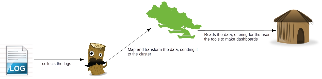
The Docker architecture consists of a client-server model, where we have a Docker client, that could be the command line one provided by Docker, or a consumer of the RESTFul API also provided on the toolset, and the Docker server, also known as Docker daemon, which receives requests to create/start/stop containers, been responsible for the container management. The diagram bellow illustrates this architecture:

On the image above we can see the Docker clients connecting to the daemon, making requests to start/stop/create containers etc. We can also see that the daemon is communicating with a image repository and using images while processing the requests. What are those images for? That’s what we will find out on the next section.

Containers & Images

When we talk about containers on Docker, we talk about processes running from instructions that were set on images. We can understand images as the building blocks from which containers are build, that way organizing the building of containers on a Docker environment.

This images are distributed on repositories, also known as a docker registry, which in turn are versioned using git. The main repository for the distribution of Docker images is, of course, the Docker Hub, managed by Docker itself.

A interesting thing is that the code behind the Docker Hub is open, so it is perfectly possible to host your own image repository. To know more about this, please visit:

github.com/docker/distribution

Docker Union File System

If the reader is familiar with traditional virtualization with hypervisors, he could be thinking: “How Docker manages the file system so the images didn’t get ‘dirt’ from the files generated on the executions of all the created containers?”. This could be even worse when we think that images can be inherited from other images, making a whole image tree.

The answer for this is how Docker utilizes the file system, with a file system called Union File System. On this system, each image is layered as a read-only layer. The layers are then overlapped on top of each other and finally on top of the chain a read-write layer is created, for the use of the container. This way, none of the image’s file systems are altered, making the images clean for use across multiple containers.

Using Docker in other OS

Docker is designed for use on Linux distributions. However, for use as a development environment, Docker inc released a Docker Toolbox that allows it to run Docker both on OSX and Windows environments as well.

In order to do this, the toolbox install virtualbox inside his distribution, as well as a micro linux VM, that only has the minimum kernel packages necessary for the launch of containers. This way, when we launch the terminal of the toolbox, the launcher starts the VM on virtualbox, starting Docker inside the VM.

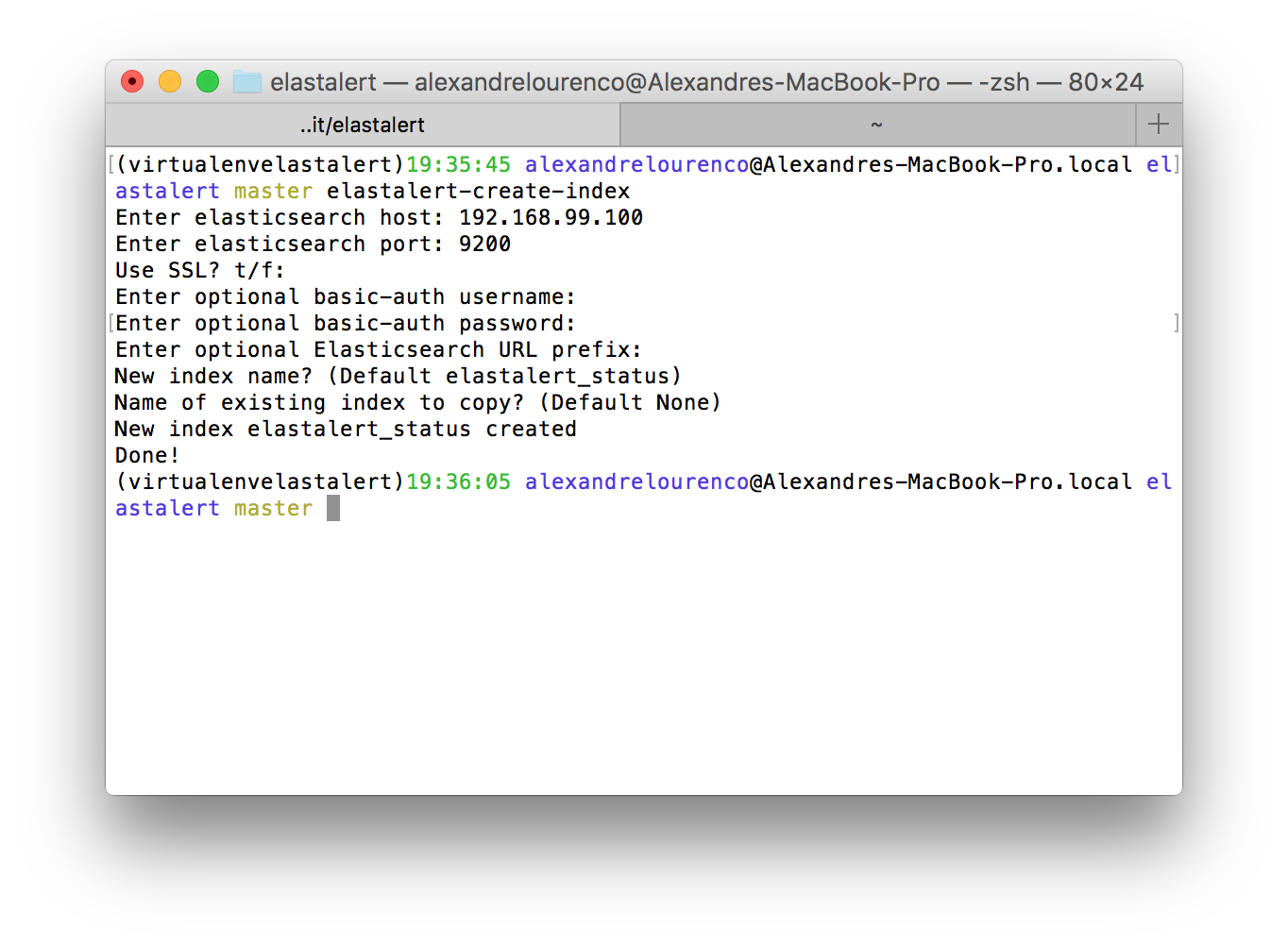
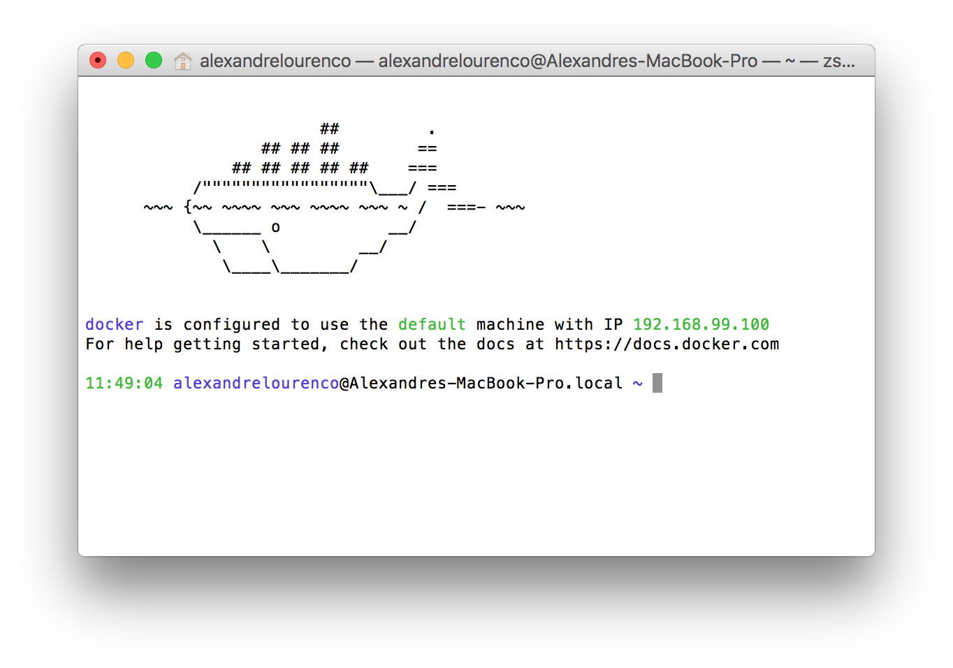
One important thing to notice is that, when we launch Docker this way, we can’t use localhost anymore when we want to access Docker from the same host it is running, since it is binded to a specific ip. We can see the ip Docker is bind to by the initialization messages, as we can see on the image bellow, from a Docker installation on OSX:

Another thing to notice is that, when we use docker on OSX or Windows, we don’t need to use sudo to execute the commands, while on Linux we will need to execute the commands as root. Another way to use Docker that removes the need to use sudo is by having a group called ‘docker’ on the machine, which will make docker apply the permissions necessary to run docker without sudo to the group. Notice, however, that users from this group will have root permissions, so caution is required.

Docker commands

Well, now that we get the concepts out of the way, let’s start using Docker!

As said before, Docker uses image repositories to resolve the images it needs to run the containers. Let’s begin by running a simple container, to make a famous ‘hello world!’, Docker style.

To do this, let’s open a terminal – or the Docker QuickStart Terminal on other OS – and type:

docker run ubuntu echo 'hello, Docker!'

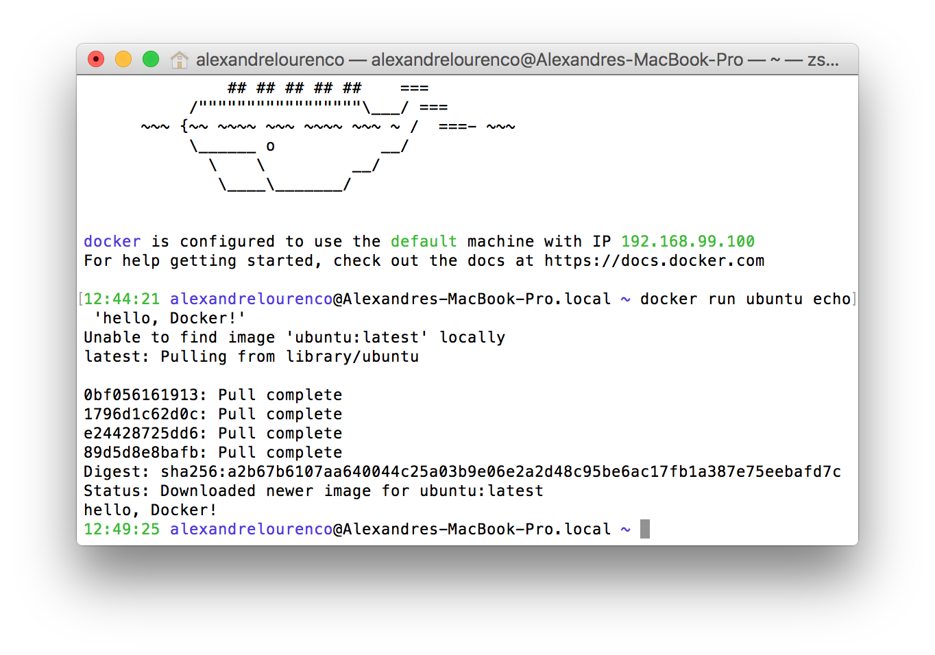
This is the run command, which creates a new container each time is called. On the command above, we simply asked Docker to create a new container, using the image ubuntu – if it doesn’t have already, Docker will search Docker Hub for the latest version of the image and download it. If we wanted to use a specific version, we could specify like this: ‘ubuntu:14.04’ – from Docker Hub. At the end, we specify a command for the container to run, on this case, a simple “echo ‘hello world!’ “.

The image bellow show the command in action, downloading the image and executing:

To list the containers created, we run the command ‘docker ps’. If we run the command this way now, however, we won’t see anything, because the command by default only shows the active containers and on our case, our container simply stopped after running the command. If we run the command with the flag -a, we can then see the stopped containers, like the image bellow:

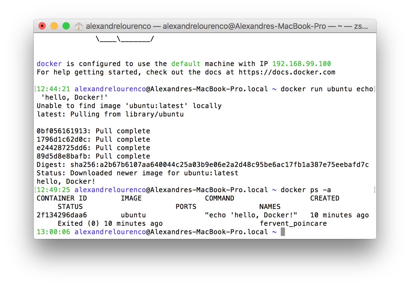
However, there’s a problem: our hello world container was just a test, so we didn’t want to keep with the container. Let’s correct this by removing the container, with the command:

docker rm 2f134296daa6

PS: The hash you can see on the command is part of the ID of the container, that you can see when you list the containers with docker ps.

Now, what about if we wanted to run again our hello world container, or any other container that we need just once, without the need to manually remove the container afterwards? We can do this using the –rm flag, running like this:

docker run --rm ubuntu echo 'hello, Docker!'

If we run docker ps -a again, after running the command above, we can see that there’s no containers from our previous execution, proving that the flag worked correctly.

Let’s now do a little more complex example, starting a container with a Tomcat server. First, let’s search for the name of the image we want on Docker Hub. To do this, open a browser and type it:

https://hub.docker.com

Once inside the Docker Hub, let’s search for the image typing ‘tomcat’ on the search box on the top right corner of the site. We will be send to a screen like the one bellow. You can see the images with some classifiers like ‘official’ and ‘automated’.

Official means that the image is maintained by Docker itself, while automated means that the image is maintained by a CI workload.On the section ‘Publishing on Docker Hub’ we will understand more about the options to publish our own images to the Docker Hub.

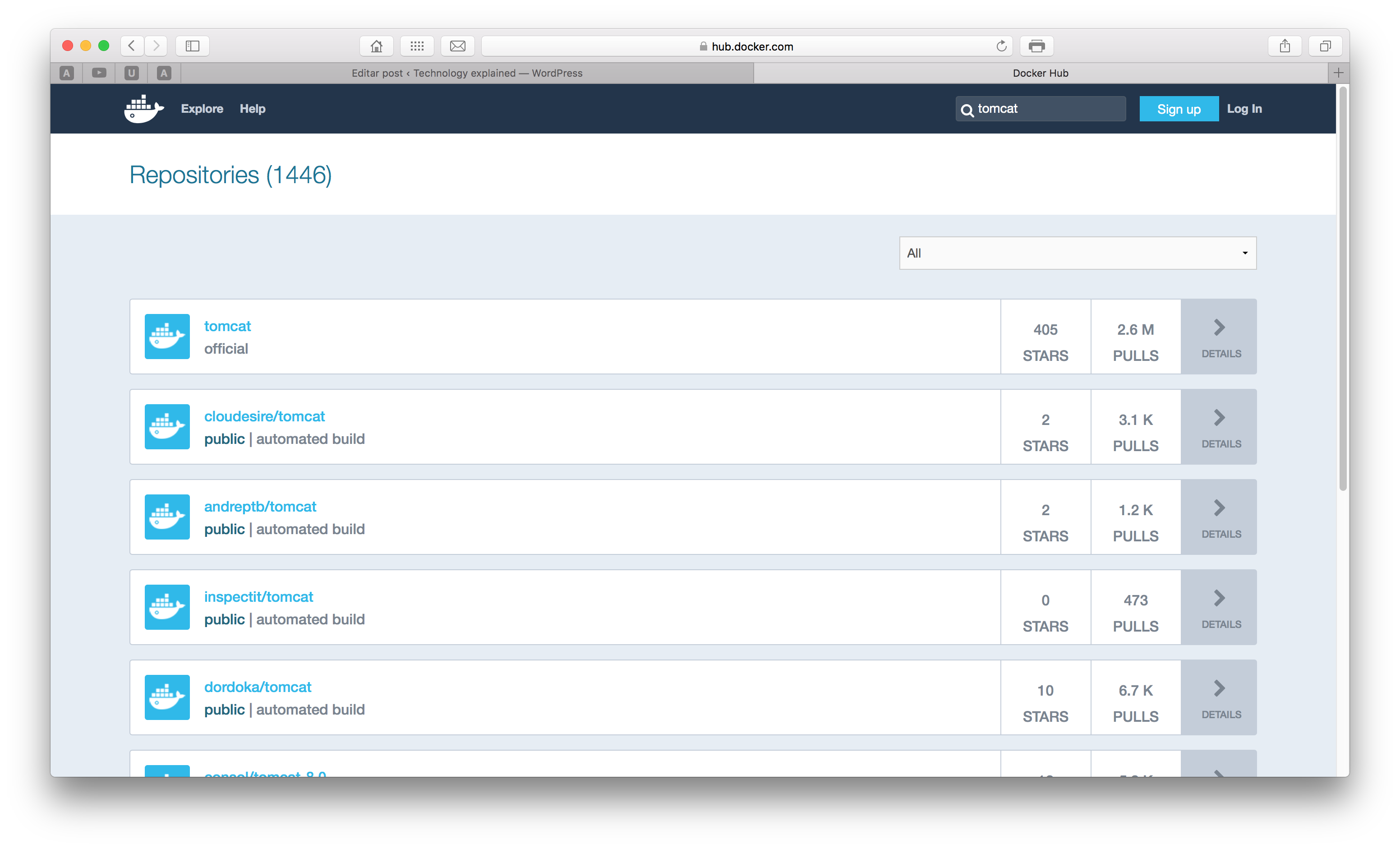
From the Docker Hub we get that the name of the official image is ‘tomcat’, so let’s use this image. To use it, we simply run the following command, which will start a new container with the tomcat image:

docker run --name mytomcat -p 8888:8080 tomcat:8.0

You can see that we used some new flags on this command. First, we used the flag –name, which makes a name for our container, so we can refer to this name when running commands afterwards.

The -p flag is used to bind a port from the host machine to a port on the container. On the next sections, we will talk about creating our own images and we will see that we can expose ports from the container to be accessed by clients, like in this case that we exposed the port tomcat will serve on the container (8080) to the port 8888 of the host.

Lastly, when declaring the image we will use, we specified the version, 8.0, meaning that we want to use Tomcat 8.0. Note that we didn’t passed any command to the container, since the image is already configured to start the Tomcat server after the building. After running the command, we can see that tomcat is running inside our container:

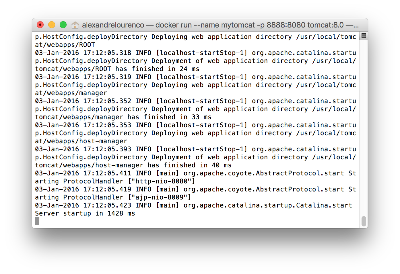
The problem is that now our terminal is occupied by the tomcat process so we can’t issue more commands. Let’s press Crtl+C and type the docker ps command. The container is not active! the reason for this is that, by default, Docker don’t put the containers to run in background when we create a new container. To do this, we use the -d flag, so on the previous command, all we had to do is include this flag to make the container start on background.

Let’s start the container again with the command docker start:

docker start mytomcat

After the start, we can see that the container is running, if we run docker ps:

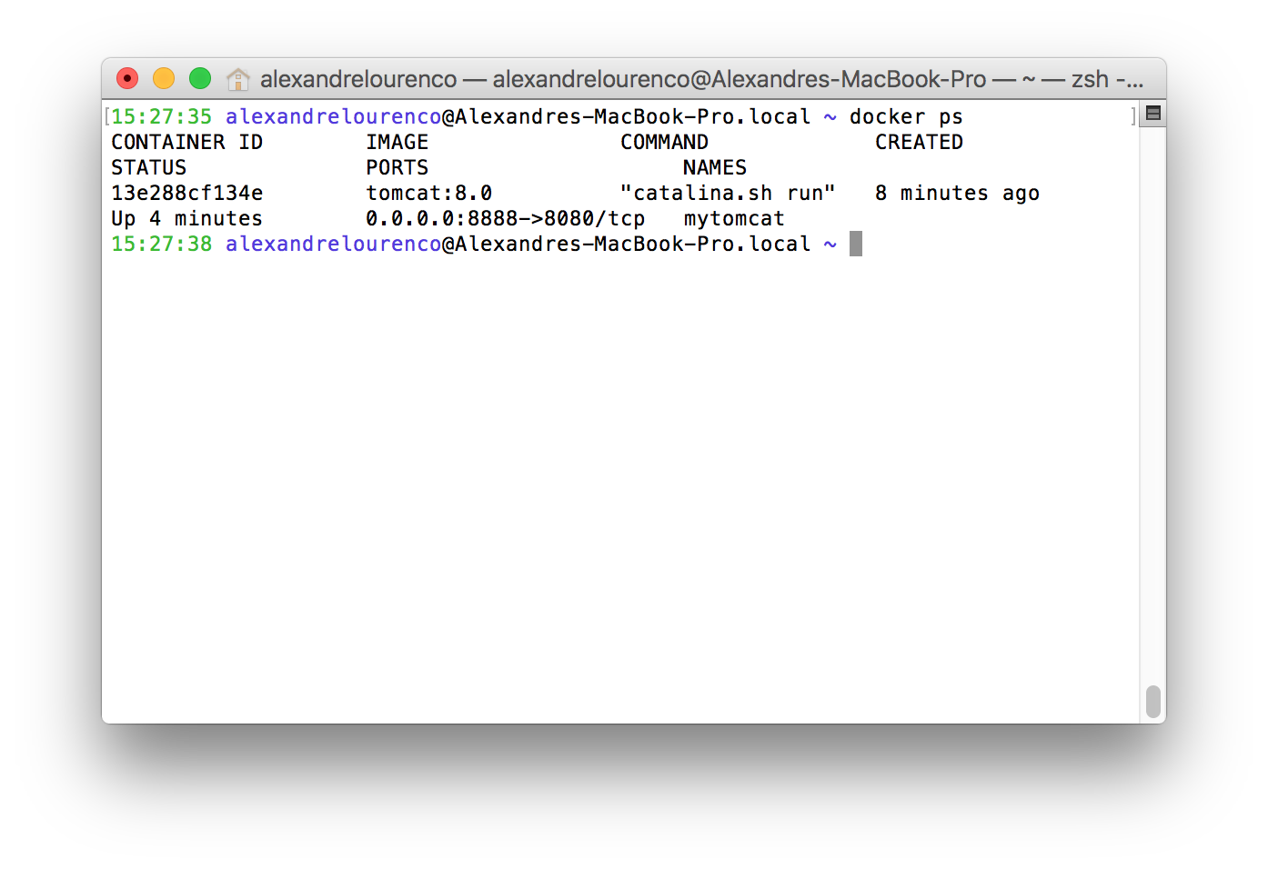
Before we open the server on the browser, let’s just check if the container is exposed on the port we defined. To do this, we use the command:

docker port mytomcat

This command will return the following result:

8080/tcp -> 0.0.0.0:8888

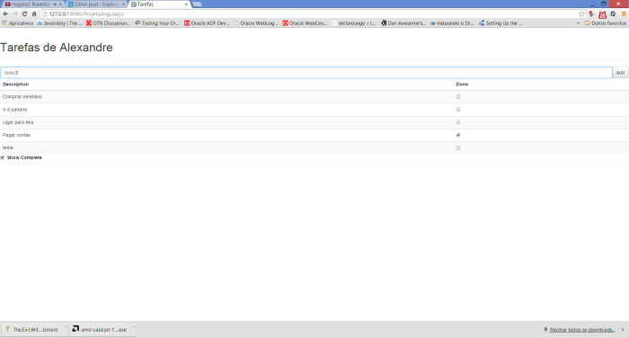
Which means that the container is exposed on the port 8888, as defined. If we open the browser on localhost:8888 – or the ip binded by Docker on a non-linux environment – we will receive the following screen:

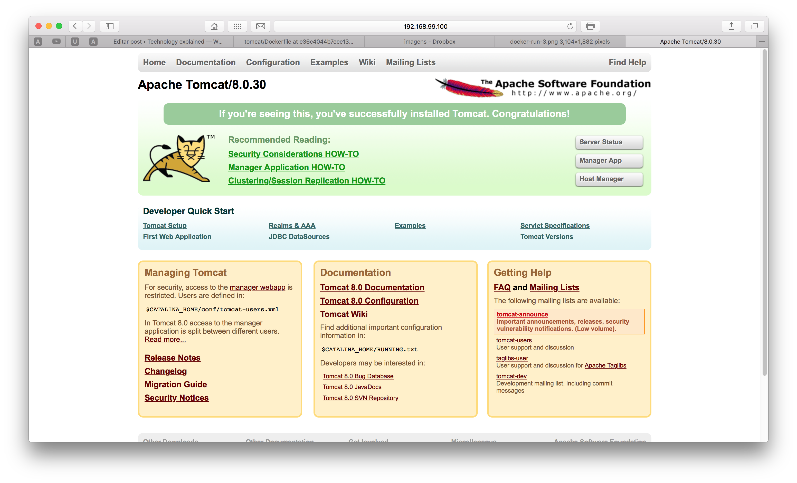
Excellent! Now we have our own dockerized Tomcat! However, by starting the container in background, we couldn’t see the logging of the server, to see if there wasn’t any problem on the startup of the web server. let’s see the last lines of the log of our container by entering the command:

docker logs mytomcat

This will show the last inputs of our container on the stdout. We could also use the command:

docker attach mytomcat

This command has the same effect of the tail command on a file, making it possible to watch the logs of the container. Take notice that after attaching to a container, pressing Ctrl+C will kill him!

Before ending our container, let’s see more detailed information about our container, such as the Java version, network mappings etc. To do this, we run the following command:

docker inspect mytomcat

This will produce a result like the following, in JSON format:

[

{

“Id”: “14598a44a3b4fe2a5b987ea365b2c83a0399f4fda476ad1754acee23c96fcc22”,

“Created”: “2016-01-03T17:59:49.632050403Z”,

“Path”: “catalina.sh”,

“Args”: [

“run”

],

“State”: {

“Status”: “running”,

“Running”: true,

“Paused”: false,

“Restarting”: false,

“OOMKilled”: false,

“Dead”: false,

“Pid”: 4811,

“ExitCode”: 0,

“Error”: “”,

“StartedAt”: “2016-01-03T17:59:49.728287604Z”,

“FinishedAt”: “0001-01-01T00:00:00Z”

},

“Image”: “af28fa31b54b2e45d53e80c5a7cbfd2693f198fdb8ba53d44d8a432832ad1012”,

“ResolvConfPath”: “/mnt/sda1/var/lib/docker/containers/14598a44a3b4fe2a5b987ea365b2c83a0399f4fda476ad1754acee23c96fcc22/resolv.conf”,

“HostnamePath”: “/mnt/sda1/var/lib/docker/containers/14598a44a3b4fe2a5b987ea365b2c83a0399f4fda476ad1754acee23c96fcc22/hostname”,

“HostsPath”: “/mnt/sda1/var/lib/docker/containers/14598a44a3b4fe2a5b987ea365b2c83a0399f4fda476ad1754acee23c96fcc22/hosts”,

“LogPath”: “/mnt/sda1/var/lib/docker/containers/14598a44a3b4fe2a5b987ea365b2c83a0399f4fda476ad1754acee23c96fcc22/14598a44a3b4fe2a5b987ea365b2c83a0399f4fda476ad1754acee23c96fcc22-json.log”,

“Name”: “/mytomcat”,

“RestartCount”: 0,

“Driver”: “aufs”,

“ExecDriver”: “native-0.2”,

“MountLabel”: “”,

“ProcessLabel”: “”,

“AppArmorProfile”: “”,

“ExecIDs”: null,

“HostConfig”: {

“Binds”: null,

“ContainerIDFile”: “”,

“LxcConf”: [],

“Memory”: 0,

“MemoryReservation”: 0,

“MemorySwap”: 0,

“KernelMemory”: 0,

“CpuShares”: 0,

“CpuPeriod”: 0,

“CpusetCpus”: “”,

“CpusetMems”: “”,

“CpuQuota”: 0,

“BlkioWeight”: 0,

“OomKillDisable”: false,

“MemorySwappiness”: -1,

“Privileged”: false,

“PortBindings”: {

“8080/tcp”: [

{

“HostIp”: “”,

“HostPort”: “8888”

}

]

},

“Links”: null,

“PublishAllPorts”: false,

“Dns”: [],

“DnsOptions”: [],

“DnsSearch”: [],

“ExtraHosts”: null,

“VolumesFrom”: null,

“Devices”: [],

“NetworkMode”: “default”,

“IpcMode”: “”,

“PidMode”: “”,

“UTSMode”: “”,

“CapAdd”: null,

“CapDrop”: null,

“GroupAdd”: null,

“RestartPolicy”: {

“Name”: “no”,

“MaximumRetryCount”: 0

},

“SecurityOpt”: null,

“ReadonlyRootfs”: false,

“Ulimits”: null,

“LogConfig”: {

“Type”: “json-file”,

“Config”: {}

},

“CgroupParent”: “”,

“ConsoleSize”: [

0,

0

],

“VolumeDriver”: “”

},

“GraphDriver”: {

“Name”: “aufs”,

“Data”: null

},

“Mounts”: [],

“Config”: {

“Hostname”: “14598a44a3b4”,

“Domainname”: “”,

“User”: “”,

“AttachStdin”: false,

“AttachStdout”: false,

“AttachStderr”: false,

“ExposedPorts”: {

“8080/tcp”: {}

},

“Tty”: false,

“OpenStdin”: false,

“StdinOnce”: false,

“Env”: [

“PATH=/usr/local/tomcat/bin:/usr/local/sbin:/usr/local/bin:/usr/sbin:/usr/bin:/sbin:/bin”,

“LANG=C.UTF-8”,

“JAVA_VERSION=7u91”,

“JAVA_DEBIAN_VERSION=7u91-2.6.3-1~deb8u1”,

“CATALINA_HOME=/usr/local/tomcat”,

“TOMCAT_MAJOR=8”,

“TOMCAT_VERSION=8.0.30”,

“TOMCAT_TGZ_URL=https://www.apache.org/dist/tomcat/tomcat-8/v8.0.30/bin/apache-tomcat-8.0.30.tar.gz”

],

“Cmd”: [

“catalina.sh”,

“run”

],

“Image”: “tomcat:8.0”,

“Volumes”: null,

“WorkingDir”: “/usr/local/tomcat”,

“Entrypoint”: null,

“OnBuild”: null,

“Labels”: {},

“StopSignal”: “SIGTERM”

},

“NetworkSettings”: {

“Bridge”: “”,

“SandboxID”: “37fe977f6a45f4495eae95260a67f0e99a8168c73930151926ad521d211b4ac6”,

“HairpinMode”: false,

“LinkLocalIPv6Address”: “”,

“LinkLocalIPv6PrefixLen”: 0,

“Ports”: {

“8080/tcp”: [

{

“HostIp”: “0.0.0.0”,

“HostPort”: “8888”

}

]

},

“SandboxKey”: “/var/run/docker/netns/37fe977f6a45”,

“SecondaryIPAddresses”: null,

“SecondaryIPv6Addresses”: null,

“EndpointID”: “09477abf22e8019e2f8d3e0deeb18d9362136954a09e336f4a93286cb3b8b027”,

“Gateway”: “172.17.0.2”,

“GlobalIPv6Address”: “”,

“GlobalIPv6PrefixLen”: 0,

“IPAddress”: “172.17.0.3”,

“IPPrefixLen”: 16,

“IPv6Gateway”: “”,

“MacAddress”: “02:42:ac:11:00:03”,

“Networks”: {

“bridge”: {

“EndpointID”: “09477abf22e8019e2f8d3e0deeb18d9362136954a09e336f4a93286cb3b8b027”,

“Gateway”: “172.17.0.2”,

“IPAddress”: “172.17.0.3”,

“IPPrefixLen”: 16,

“IPv6Gateway”: “”,

“GlobalIPv6Address”: “”,

“GlobalIPv6PrefixLen”: 0,

“MacAddress”: “02:42:ac:11:00:03”

}

}

}

}

]

Now, let’s stop our container, by entering:

docker stop mytomcat

Finally, let’s remove the container, since we won’t use him anymore on this practice:

docker rm mytomcat

Let’s also remove the image, since we won’t use it either on our next steps:

docker rmi tomcat:8.0

And that concludes our breaking course on Docker’s commands! There are also other useful commands as well, of course, such as:

docker build: Used to build a image from a Dockerfile (see next sections);
docker commit: Creates a image from a container;
docker push: Pushes the image for a registry (Docker Hub by default);
docker exec: Submit a command for a running container;
docker export: Export the file system of a container as a tar file;
docker images: list the images inside Docker;
docker kill: force kill a running container;
docker restart: restart a container;
docker network: manages docker networks (see next sections);
docker volume: manages docker volumes (see next sections);

Creating your own images

On the previous section, we used a image from the Docker Hub, that creates a container with a Tomcat Web Server. This image is implemented by a script with building instructions called Dockerfile. On our lab we will create a Dockerfile, but for now, let’s just examine the Dockerfile from the tomcat’s image in order to learn some of the instructions available:

FROM java:7-jre
ENV CATALINA_HOME /usr/local/tomcat

ENV PATH $CATALINA_HOME/bin:$PATH

RUN mkdir -p “$CATALINA_HOME”

WORKDIR $CATALINA_HOME
# see https://www.apache.org/dist/tomcat/tomcat-8/KEYS

RUN gpg –keyserver pool.sks-keyservers.net –recv-keys \

05AB33110949707C93A279E3D3EFE6B686867BA6 \

07E48665A34DCAFAE522E5E6266191C37C037D42 \

47309207D818FFD8DCD3F83F1931D684307A10A5 \

541FBE7D8F78B25E055DDEE13C370389288584E7 \

61B832AC2F1C5A90F0F9B00A1C506407564C17A3 \

79F7026C690BAA50B92CD8B66A3AD3F4F22C4FED \

9BA44C2621385CB966EBA586F72C284D731FABEE \

A27677289986DB50844682F8ACB77FC2E86E29AC \

A9C5DF4D22E99998D9875A5110C01C5A2F6059E7 \

DCFD35E0BF8CA7344752DE8B6FB21E8933C60243 \

F3A04C595DB5B6A5F1ECA43E3B7BBB100D811BBE \

F7DA48BB64BCB84ECBA7EE6935CD23C10D498E23
ENV TOMCAT_MAJOR 8

ENV TOMCAT_VERSION 8.0.30

ENV TOMCAT_TGZ_URL https://www.apache.org/dist/tomcat/tomcat-$TOMCAT_MAJOR/v$TOMCAT_VERSION/bin/apache-tomcat-$TOMCAT_VERSION.tar.gz
RUN set -x \

&& curl -fSL “$TOMCAT_TGZ_URL” -o tomcat.tar.gz \

&& curl -fSL “$TOMCAT_TGZ_URL.asc” -o tomcat.tar.gz.asc \

&& gpg –verify tomcat.tar.gz.asc \

&& tar -xvf tomcat.tar.gz –strip-components=1 \

&& rm bin/*.bat \

&& rm tomcat.tar.gz*
EXPOSE 8080

CMD [“catalina.sh”, “run”]

As we can see, the first instruction is called FROM. This instruction delimits the base image upon the image will be constructed. On this case, the java:7-jre image will create a basic Linux environment, with Java 7 configured.

Then we see some ENV instructions. This commands set environment variables on the OS, as part of Tomcat’s configuration. We can also see a WORKDIR instruction, which defines the directory that, from that point, Docker will use to run the commands.

We also see some RUN instructions. This instructions, as the name implies, run commands on the container.On the case of our image, this instructions make tomcat’s installation process.

Finally we see the EXPOSE instruction, which exposes the 8080 port for the host. Finally, we see the CMD instruction, which defines the start of the server. One important distinction of the CMD command from the RUN ones is that, while the RUN instructions only executes on the build phase, the CMD instruction is executed on the container’s startup, making it the command to be executed on the creation and start of a container. For this reason, it is only allowed to have one CMD command per Dockerfile.

One important side note about the CMD command is that, when starting a container, it allows to override the command on the Dockerfile, so it could lead to security holes when used. For this reason, it is recommended to use the ENTRYPOINT instruction instead, that like the CMD instruction, it defines the command the container will run at startup, but on this case, it will not permit the command to be overridden, making it more secure.

We could also use ENTRYPOINT and CMD combined, making it possible to restrict the user to only pass flags and/or arguments to the running command.

Of course, that is not the only instructions we can use on a Dockerfile. Other instructions are:

MAINTAINER: Defines the author of the image;
LABEL: Adds metadata to a image, in a key=value format;
ADD: Adds a file, folder or remote file URL to a folder inside the container. The current directory from which this instruction point it out is the same directory of the Dockerfile;
COPY: Analogous to ADD, this instruction also copies files and folders from the host to the container. The two major differences are that COPY doesn’t allow the use of URLs and COPY doesn’t uncompress known files, like ADD can;
VOLUME: Creates a volume. On the section “creating the base image” we will learn in more detail about what are volumes on Docker;
USER: Defines the name of the user used to run the RUN, CMD and ENTRYPOINT instructions;
ARG: Defines build-time variables, that could be used to pass parameters for the image’s buildings, using the —build-arg flag;
ONBUILD: Defines a command to be triggered by other images, when the image is used as a base image for other images;
STOPSIGNAL: Defines the code for the container to stop, as a number or in the SIGNAME format, for instance SIGKILL.

Publishing on Docker Hub

As we saw on the previous section, in order to create our own images, all we have to do is create a “Dockerfile” file, with the instructions necessary for the building. However, in order to distribute our images, we need to register them on a image registry, like the Docker Hub, for example.

The simplest way to publish images are with the commit and push commands. For example, if we had made changes to our Tomcat container and wanted to save those changes as a new image, we could do this with this command:

docker commit mytomcat alexandreesl/mytomcat

Where the second argument is the <repository ID>/<image name>. In order to push the images to Docker Hub, the repository ID must be equals to the username of our Docker Hub account.

After committing the changes, all we have to do is push the changes to the Hub, using the following command:

docker push alexandreesl/mytomcat

And that’s it! After the push, if we see our Docker Hub account, we can see that our image was successfully created:

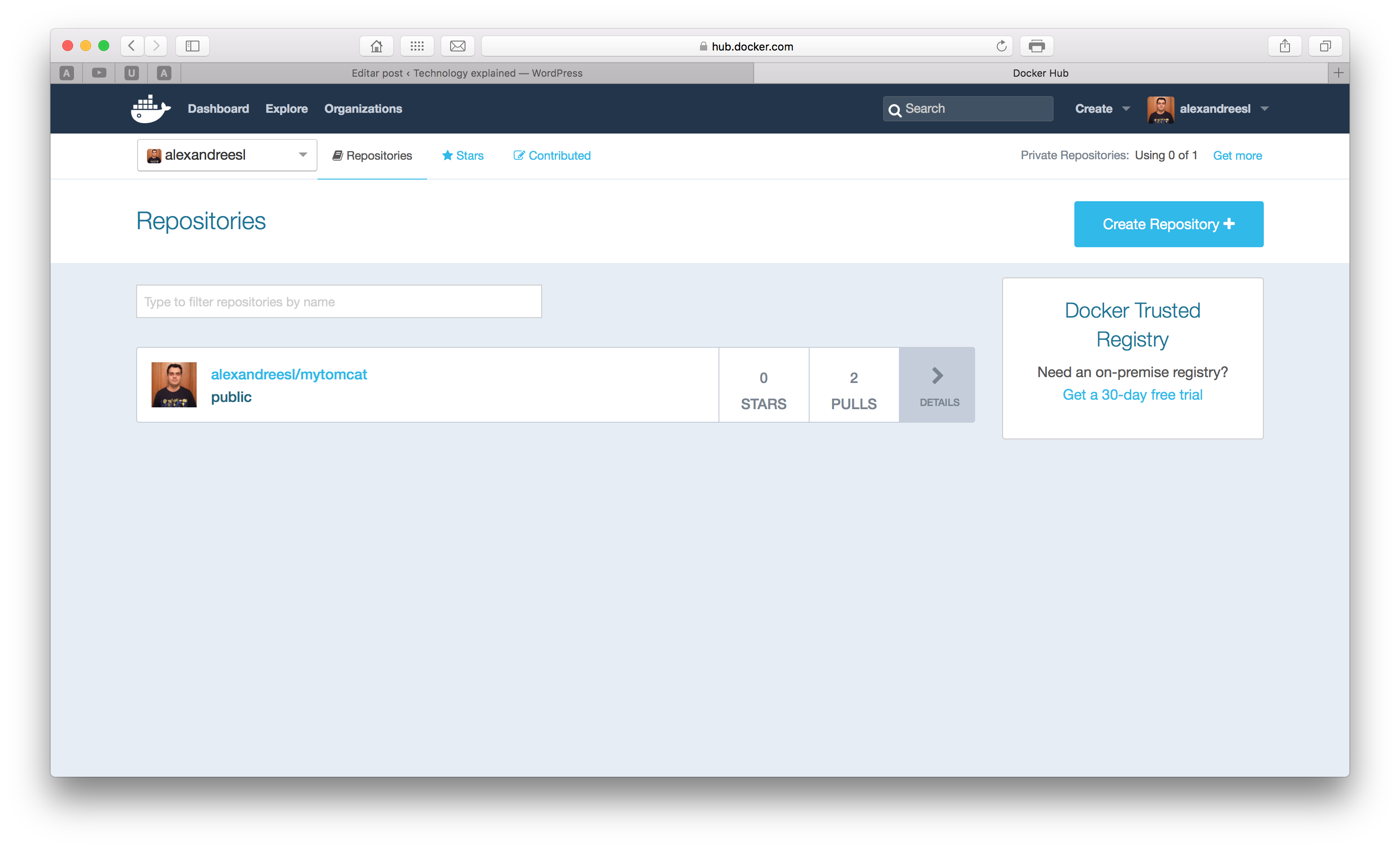
NOTE: before pushing, you could have to run the command docker login to register your credentials from the Docker Hub

Another way of publishing is by linking our images with a git repository, this way the Docker Hub will rebuild the image each time a new version of the Dockerfile is pushed to the repository. Is this method of publishing that generates automated build images, since this way Docker can establish a CI Workload with the git repository. We will see this method in action on the next section, ‘Creating the base image’.

Practice: Using Docker to implement a microservices architecture

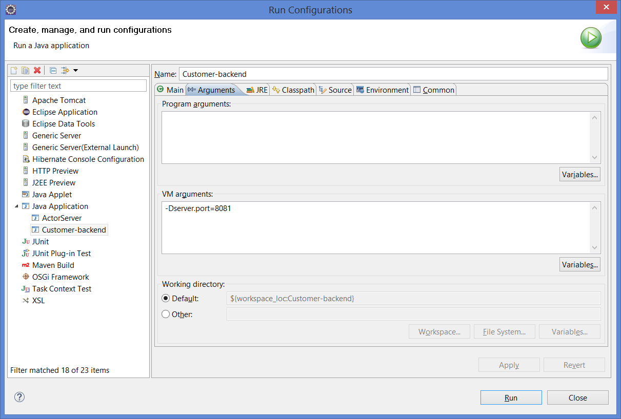
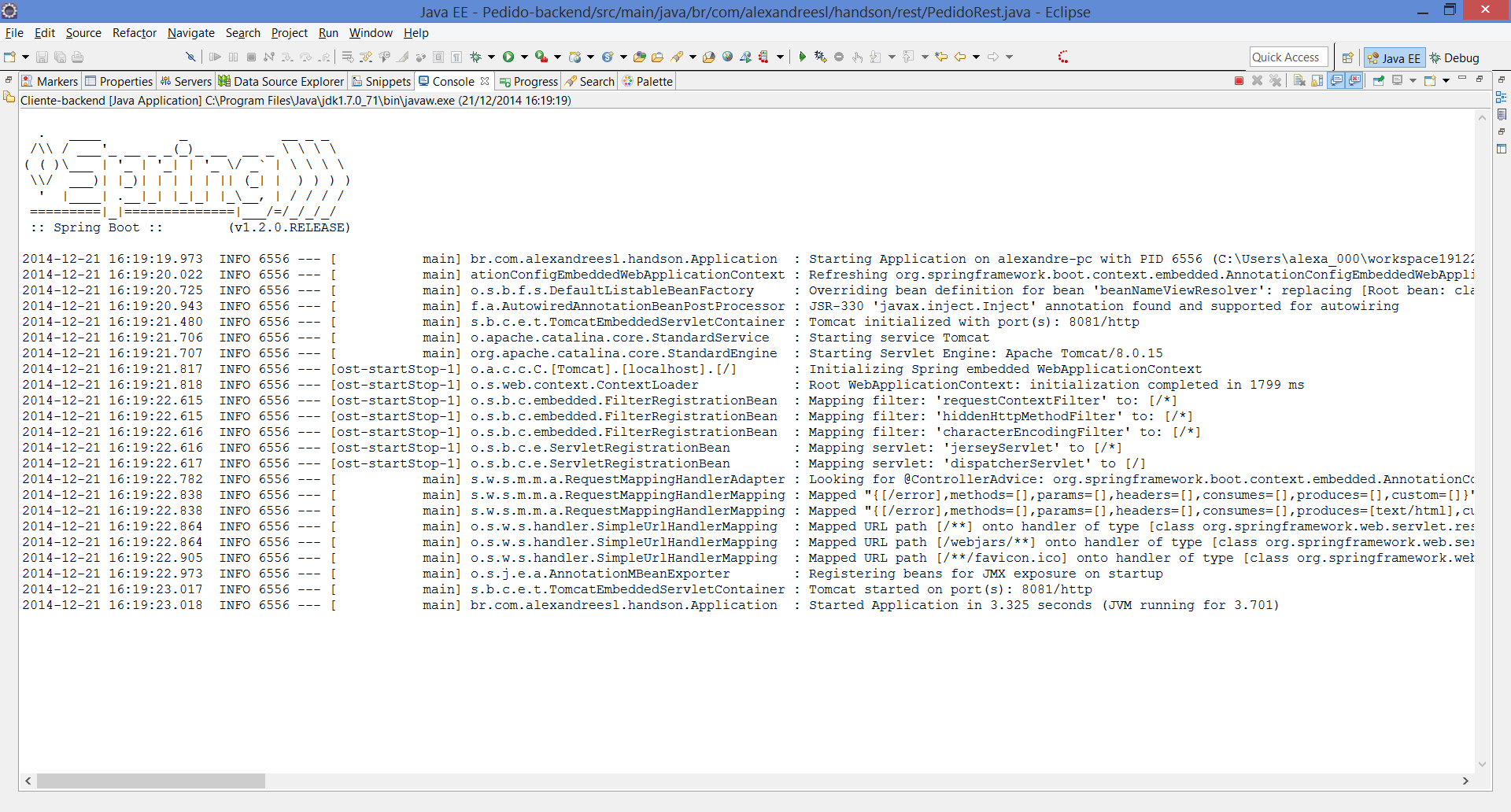
On our lab, we will take a step forward from my previous post about microservices with Spring Boot (haven’t see it? you can find it here, I am really grateful if you read that post as well!), by using a Service Registry called Eureka, designed by Netflix.

On the Service Registry pattern, we have a registry where microservices can register/unregister and also find the addresses of a service dynamically, this way decoupling the bounds between them. We will dockerize (run inside a container) the services of that lab and make them use Eureka, which will also run inside a container. In order to integrate with Eureka, we will modify our applications to use the Spring Cloud project, which according to the project’s description:

Spring Cloud provides tools for developers to quickly build some of the common patterns in distributed systems (e.g. configuration management, service discovery, circuit breakers, intelligent routing, micro-proxy, control bus, one-time tokens, global locks, leadership election, distributed sessions, cluster state). Coordination of distributed systems leads to boiler plate patterns, and using Spring Cloud developers can quickly stand up services and applications that implement those patterns. They will work well in any distributed environment, including the developer’s own laptop, bare metal data centres, and managed platforms such as Cloud Foundry.

Also, to “Springfy” even more our example, we will exchange our implementation from the previous post that uses pure jax-rs to the RestController implementation, present on the Spring Web project.

Creating the base image

Well, so let’s begin our practice! First, we will create a Docker Network to accommodate the containers.

If we see the network adapters from the host machine when the Docker Daemon is up, we will see that he creates a bridge adapter on the host, subsequently appending the containers on network interfaces inside the bridge adapter. This forms a subnet where the containers can see each other and also Docker facilitates the work for us, by mapping the container’s IPs with their names, on the /etc/hosts files inside.

On our scenario, we will use this feature so the microservices can easily find our Eureka registry, by mapping the address to the container’s name. Of course that on a real scenario we would have a cluster of Eurekas with a load balancer on separate hosts, but for simplicity’s sake of our lab, we will just use one Eureka instance.

So, in order to create a network to accommodate our architecture, first we create a network, by running the following command:

docker network create microservicesnet

After running the command we will see a hash’s ID indicating our network was created. We can see the details of our network by running the following command:

docker network inspect microservicesnet

Which will produce a result like the following:

[

{

“Name”: “microservicesnet”,

“Id”: “e8d401a00de26b74f4f2461c13dbf848c14f37127b3337a3e40465eff5897910”,

“Scope”: “local”,

“Driver”: “bridge”,

“IPAM”: {

“Driver”: “default”,

“Config”: [

{}

]

},

“Containers”: {},

“Options”: {}

}

]

Notice that, for now, the containers object is empty. This is why we didn’t add any containers to the network yet, but this will soon change.

Now we will create the Dockerfile. Create a folder in the directory of your choice and create a file called ‘Dockerfile’ (without any extension). On my case, I will push my Dockerfile to a Github repository, in order to create the image on Docker Hub as a automated build image. You can find the repositories with the source for this lab at the end of the post.

So, without further delay, let’s code the Dockerfile. The code for our image will be the following:

FROM java:8-jre

MAINTAINER Alexandre Lourenco <alexandreesl@example.com>

VOLUME [ "/data" ]

WORKDIR /data

EXPOSE 8080
ENTRYPOINT [ "java" ]
CMD ["-?"]

As we can see, it is a simple Dockerfile. We use Java’s 8 official image as the base, define a volume and set his folder as our Workdir, expose the 8080 port which is the default for Spring Boot and finally we combine the entrypoint and cmd commands, meaning that anything we pass when we get up a container will be treated as parameters for the Java command. But what is this volume we have speaked of?

The reader must remember what we saw about the Union File System and how each image is layered as a read-only layer. The volumes on Docker is a technique that bypasses the Union File System, by defining a mount point on the Containers that points for a shared space on the host machine. The uses of this technique are in order to provide a place where the container can read/write information that needs to be persisted, alongside the need to share data between containers.

On our scenario, we will use the volume to point to a place where the jars of our microservices will be generated, so when a container runs a microservice, it runs the last version of the software. On a real-world scenario, this place could be a result of a CI workload, for example from a Jenkins job.

Now that we have our image, let’s build the image to test his correctness:

docker build -t alexandreesl/microservices-spring-boot-base .

At the end, we will see a message that our building was successful, validating the Dockerfile. Out of curiosity, if you see the building process, you will notice that Docker created several temporary containers for each instruction of our script, maintaining a status of the last successful instruction executed, so if we have to rebuild the image after a failure, we can restart from the failed point. We can disable this feature with the flag -no-cache if we want.

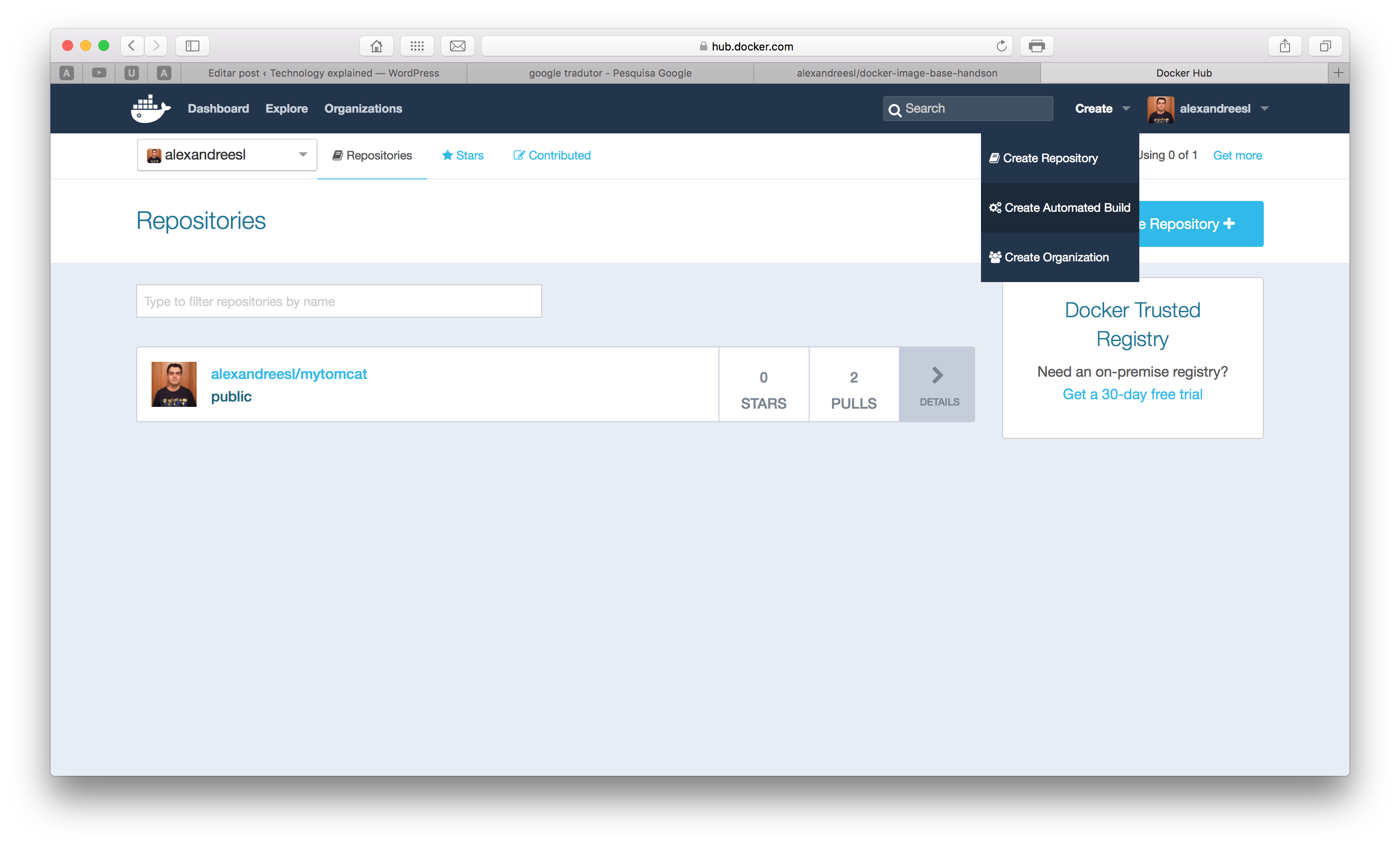
Now, let’s register the image on Docker Hub. I have created a Github repository here, so I will register the image directly on the site. To do this, we log in on our account and click on the “create automated build” menu item, as shown on the screen bellow:

After clicking, if we haven’t linked a github account yet, we will be prompted to do so. after making the linking, we will see a page with the list of our git repositories. We select the one with the Dockerfile and finally create the image, entering the name and a description for the image, as the screen bellow:

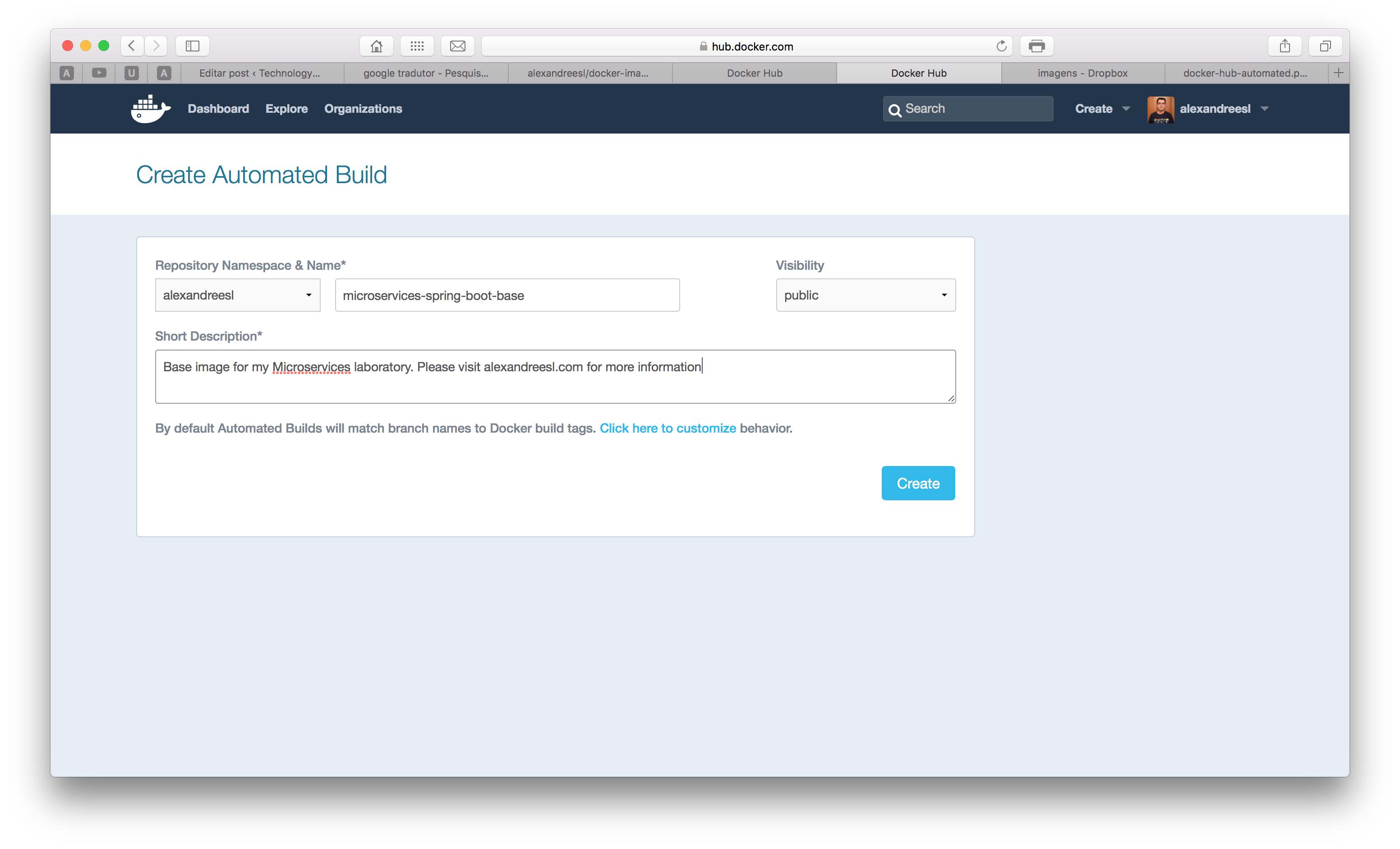
After clicking on the create button, we have completed our step, successfully registering our image on the Docker Hub! You can see my image on this link.

Lastly, just to test if our Docker Hub upload was really successful, we will remove the image from the local cache – that we added with our docker build command – and download using the docker pull command. First, let’s remove the image with the command:

docker rmi alexandreesl/microservices-spring-boot-base

And after, let’s pull the image with the command:

docker pull alexandreesl/microservices-spring-boot-base

After the download, we will have the image from the Docker Hub repository.

Preparing the service registry image

For the service registry image, we actually don’t have to do any coding, since we will use a already made image. We will start the image on the “Launching the containers” section, but the reader can see the image’s page to satisfy his curiosity here.

Preparing the services to use the registry

Now, Let’s prepare the services for the registering/deregistering of microservices, alongside service discovery when a service has dependencies.

To focus on the explanation, I will omit some details like the pom configuration, since the reader can easily get the configuration on the Github repository from the lab. On this lab, we have 3 microservices: a Customer service, a Product service and a Order service. The Order service has dependencies on the other 2 services, in order to mount a Order.

On the 3 projects we will have the same configuration for Spring Boot’s main class, called Application, as follows:

@SpringBootApplication
@Configuration
@EnableAutoConfiguration
@EnableEurekaClient
public class Application {

public static void main(String[] args) {
 SpringApplication.run(Application.class, args);
 }
}

The key line here is the annotation @EnableEurekaClient, which configures the Spring Boot’s application to work with Eureka. Just with these annotation alone, we configure Spring Boot to connect to Eureka at startup and register itself with, send heartbeats during his lifecycle to keep the registration alive and finally make a unregistration when the process is terminated. Also, it instantiate a RestTemplate with a Ribbon load balancer, also made by Netflix, that can easily lookup service addresses from the registry. All of this with just one annotation!

In order to connect to Eureka, we have to provide the registry’s address. this is made by configuring a YAML file, called application.yml, that we put it on the resources source folder. We also configure a application name on this file, in order to inform Eureka about what Application’s ID we would like to use for the microservice.

So, in order to make this configuration, we create the files on our projects. seeing a example, for the Order’s service, we have the following YAML configuration:

spring:
 application:
 name: OrderService
eureka:
 client:
 serviceUrl:
 defaultZone: http://eureka:8761/eureka/

Notice that when we configure Eureka’s address, we used “eureka” as the host name. This is the name of the container that we will use in order to deploy the Eureka server on our Docker Network, so on the /etc/hosts files of our containers, this name will be mapped to Eureka’s container IP, making it possible to point it out dynamically.

Now let’s see how our Microservices were implemented. For the Customer service, we have the following code:

@RestController
@RequestMapping("/")
public class CustomerRest {

private static List<Customer> clients = new ArrayList<Customer>();

static {
Customer customer1 = new Customer();
 customer1.setId(1);
 customer1.setName("Cliente 1");
 customer1.setEmail("customer1@gmail.com");

Customer customer2 = new Customer();
 customer2.setId(2);
 customer2.setName("Cliente 2");
 customer2.setEmail("customer2@gmail.com");

Customer customer3 = new Customer();
 customer3.setId(3);
 customer3.setName("Cliente 3");
 customer3.setEmail("customer3@gmail.com");

Customer customer4 = new Customer();
 customer4.setId(4);
 customer4.setName("Cliente 4");
 customer4.setEmail("customer4@gmail.com");

Customer customer5 = new Customer();
 customer5.setId(5);
 customer5.setName("Cliente 5");
 customer5.setEmail("customer5@gmail.com");

clients.add(customer1);
 clients.add(customer2);
 clients.add(customer3);
 clients.add(customer4);
 clients.add(customer5);
}

@RequestMapping(method = RequestMethod.GET, produces = MediaType.APPLICATION_JSON_VALUE)
 public List<Customer> getClientes() {
 return clients;
 }

@RequestMapping(value = "customer/{id}", method = RequestMethod.GET, produces = MediaType.APPLICATION_JSON_VALUE)
 public Customer getCliente(@PathVariable long id) {

Customer cli = null;

for (Customer c : clients) {

if (c.getId() == id)
 cli = c;

}

return cli;
 }
}

As we can see, nothing out of normal, very simple usage of Spring’s REST Controllers. Now, on to the Product service:

@RestController
@RequestMapping("/")
public class ProductRest {

private static List<Product> products = new ArrayList<Product>();

static {

Product product1 = new Product();
 product1.setId(1);
 product1.setSku("abcd1");
 product1.setDescription("Produto1");

Product product2 = new Product();
 product2.setId(2);
 product2.setSku("abcd2");
 product2.setDescription("Produto2");

Product product3 = new Product();
 product3.setId(3);
 product3.setSku("abcd3");
 product3.setDescription("Produto3");

Product product4 = new Product();
 product4.setId(4);
 product4.setSku("abcd4");
 product4.setDescription("Produto4");

products.add(product1);
 products.add(product2);
 products.add(product3);
 products.add(product4);

}

@RequestMapping(method = RequestMethod.GET, produces = MediaType.APPLICATION_JSON_VALUE)
 public List<Product> getProdutos() {
 return products;
 }

@RequestMapping(value = "product/{id}", method = RequestMethod.GET, produces = MediaType.APPLICATION_JSON_VALUE)
 public Product getProduto(@PathVariable long id) {

Product prod = null;

for (Product p : products) {

if (p.getId() == id)
 prod = p;

}

return prod;
 }

}

Again, nothing unusual on the code. Now, let’s see the Order service, where we will see the registry been used for consuming microservices:

@RestController
@RequestMapping("/")
public class OrderRest {

private static long id = 1;

// Created automatically by Spring Cloud
 @Autowired
 @LoadBalanced
 private RestTemplate restTemplate;

private Logger logger = Logger.getLogger(OrderRest.class);

@RequestMapping(value = "order/{idCustomer}/{idProduct}/{amount}", method = RequestMethod.GET, produces = MediaType.APPLICATION_JSON_VALUE)
 public Order submitOrder(@PathVariable long idCustomer, @PathVariable long idProduct, @PathVariable long amount) {

Order order = new Order();

 Map map = new HashMap();

 map.put("id", idCustomer);

ResponseEntity<Customer> customer = restTemplate.exchange("http://CUSTOMERSERVICE/customer/{id}",
 HttpMethod.GET, null, Customer.class, map);

 map = new HashMap();

 map.put("id", idProduct);

ResponseEntity<Product> product = restTemplate.exchange("http://PRODUCTSERVICE/product/{id}", HttpMethod.GET,
 null, Product.class, map);

order.setCustomer(customer.getBody());
order.setProduct(product.getBody());
order.setId(id);
order.setAmount(amount);
order.setOrderDate(new Date());

logger.warn("The order " + id + " for the client " + customer.getBody().getName() + " with the product "
 + product.getBody().getSku() + " with the amount " + amount + " was created!");

id++;

return order;
 }
}

The first thing we notice is the autowired RestTemplate, that also has a@LoadBalanced annotation. This RestTemplate is automatically instantiated by Spring Cloud, creating a interface which we could use to communicate with Eureka. The annotation informs that we want to use Ribbon to make the load balance, in case we have a cluster of instances of the same service.

The exchange method we use inside of the submitOrder method is where the magic happens. When we make our calls using this method, internally a lookup is made with the Eureka Server, the addresses of the service are passed to Ribbon in order to load balance the calls, and them the call is made. Notice that we used names like “CUSTOMERSERVICE” as the host address on our URIs. This pattern tells the framework the ID of the application we really want to call, been replaced at runtime with one of the IP addresses of the service we want to call.

And that concludes our quick explanation of the Java code involved on our lab. Again, if the reader want to get the full code, just head for the Github repositories at the end of this post. In order to run the lab, I recommend that you clone the whole repository and execute a mvn package command on each of the 3 projects. If you don’t have Maven, you can get it from here.

Launching the containers

Now that we are almost finished with the lab, it is time for the fun part: run our containers! To do this, we will use docker-compose. With docker-compose, we can start/stop/kill etc full stacks of containers, without having to instantiate everything by hand. In order to make our docker-compose stack, let’s create a YAML file called docker-compose.yml and include the following configuration:

eureka:
 image: springcloud/eureka
 container_name: eureka
 ports:
 - "8761:8761"
 net: "microservicesnet"
customer1:
 image: alexandreesl/microservices-spring-boot-base
 container_name: customer1
 hostname: customer1
 net: "microservicesnet"
 ports:
 - "8080:8080"
 volumes:
 - /Users/alexandrelourenco/Applications/git/docker-handson:/data
 command: -jar /data/Customer-backend/target/Customer-backend-1.0.jar
product1:
 image: alexandreesl/microservices-spring-boot-base
 container_name: product1
 hostname: product1
 net: "microservicesnet"
 ports:
 - "8081:8080"
 volumes:
 - /Users/alexandrelourenco/Applications/git/docker-handson:/data
 command: -jar /data/Product-backend/target/Product-backend-1.0.jar
order1:
 image: alexandreesl/microservices-spring-boot-base
 container_name: order1
 hostname: order1
 net: "microservicesnet"
 ports:
 - "8082:8080"
 volumes:
 - /Users/alexandrelourenco/Applications/git/docker-handson:/data
 command: -jar /data/Order-backend/target/Order-backend-1.0.jar

Some things to notice from our configuration:

In all the containers we configured our “microservicesnet” network, in order to use the Docker Network feature to resolve our needs;
On the MicroService’s containers, we also defined the hostname, to force Spring Cloud’s registration control to properly register the correct alias for the service’s addresses;
We have exposed Eureka’s port to the physical host at 8761, so we can see the web interface from outside the Docker environment;
On the volumes sections, I have mapped the base folder where my Maven projects from the microservices are placed, binding to the /data folder inside the container, which is defined as the workdir on the image we created previously. This way, on the command section, when we map the location of the microservice’s Spring Boot jar, we map the location from the /data folder;

Finally, after saving our file, we run the script by simply running the following command, at the same folder of the YAML file:

docker-compose up

We will see some information about our containers getting up and at the end we will see some log information from all the containers mixed, with the name of the container as a prefix for identification:

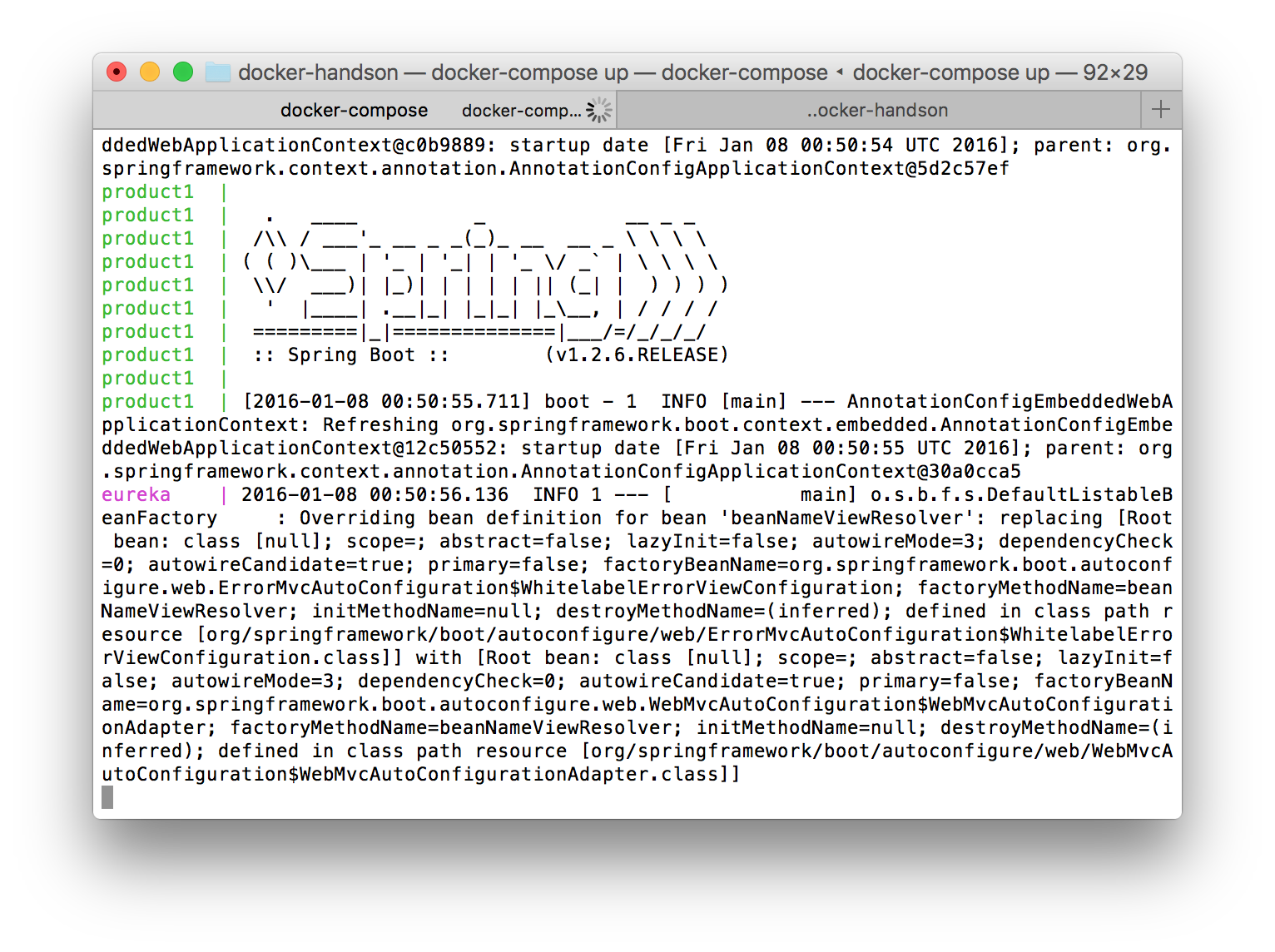
After waiting some moments we will see our containers are up. Let’s see if the microservices are up? Let’s open a browser and point it to the port 8761, using localhost or the ip used by Docker in case you are in OSX/Windows:

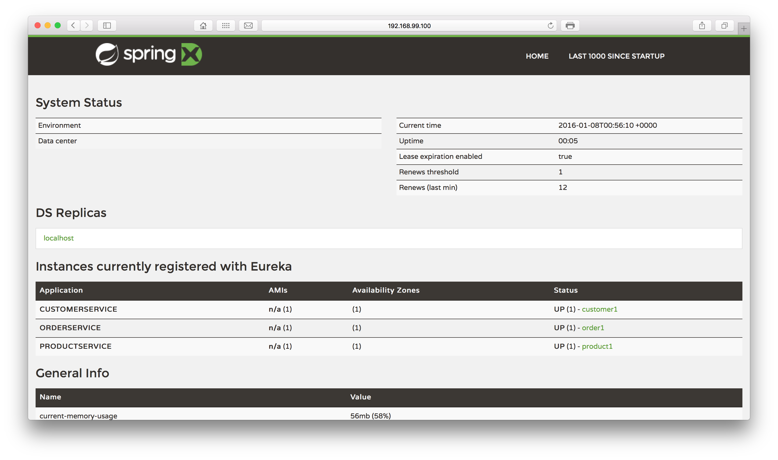
Excellent! Not only has Eureka booted up successfully, but also all of our services have registered with it. Let’s now toy a little with our stack, to test it out.

Let’s begin by making a search for a customer of ID 1 on the Customer’s service:

curl -XGET 'http://<your ip>:8080/customer/1'

This will produce a JSON response like the following:

{"id":1,"name":"Cliente 1","email":"customer1@gmail.com"}

Next, let’s test out the Product service, with a call for the details of the Product of ID 4:

curl -XGET 'http://<your ip>:8081/product/4'

This time it will produce a response like the following:

{"id":4,"sku":"abcd4","description":"Produto4"}

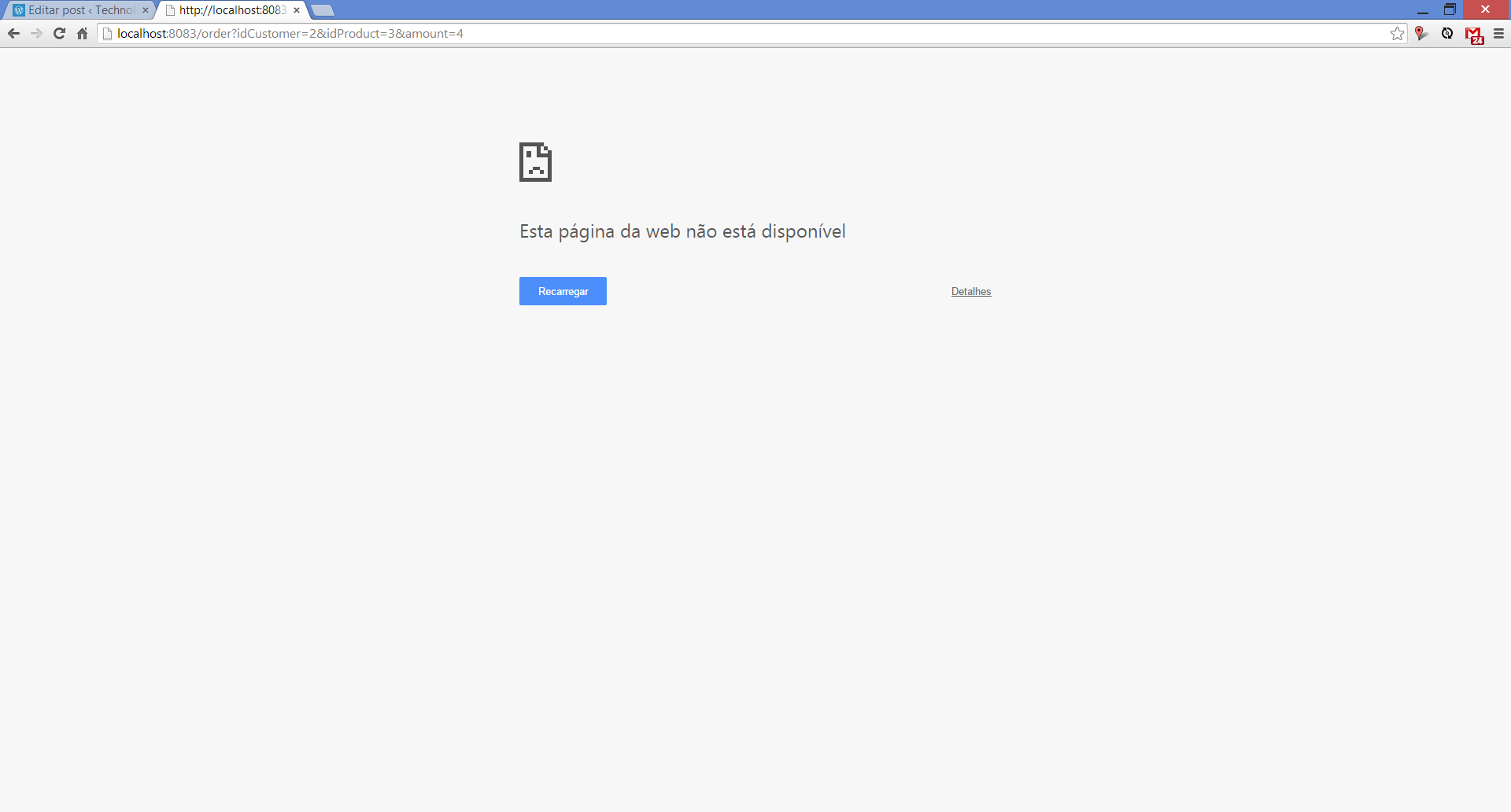
Finally, the moment of true: let’s call the Order service, that utilises our other 2 services, to see if the service’s addresses are resolved with Eureka’s help. To test it, let’s make the following call:

curl -XGET 'http://<your ip>:8082/order/2/1/4'

If everything goes well, we will see a response like:

{"id":1,"amount":4,"orderDate":1452216090392,"customer":{"id":2,"name":"Cliente 2","email":"customer2@gmail.com"},"product":{"id":1,"sku":"abcd1","description":"Produto1"}}

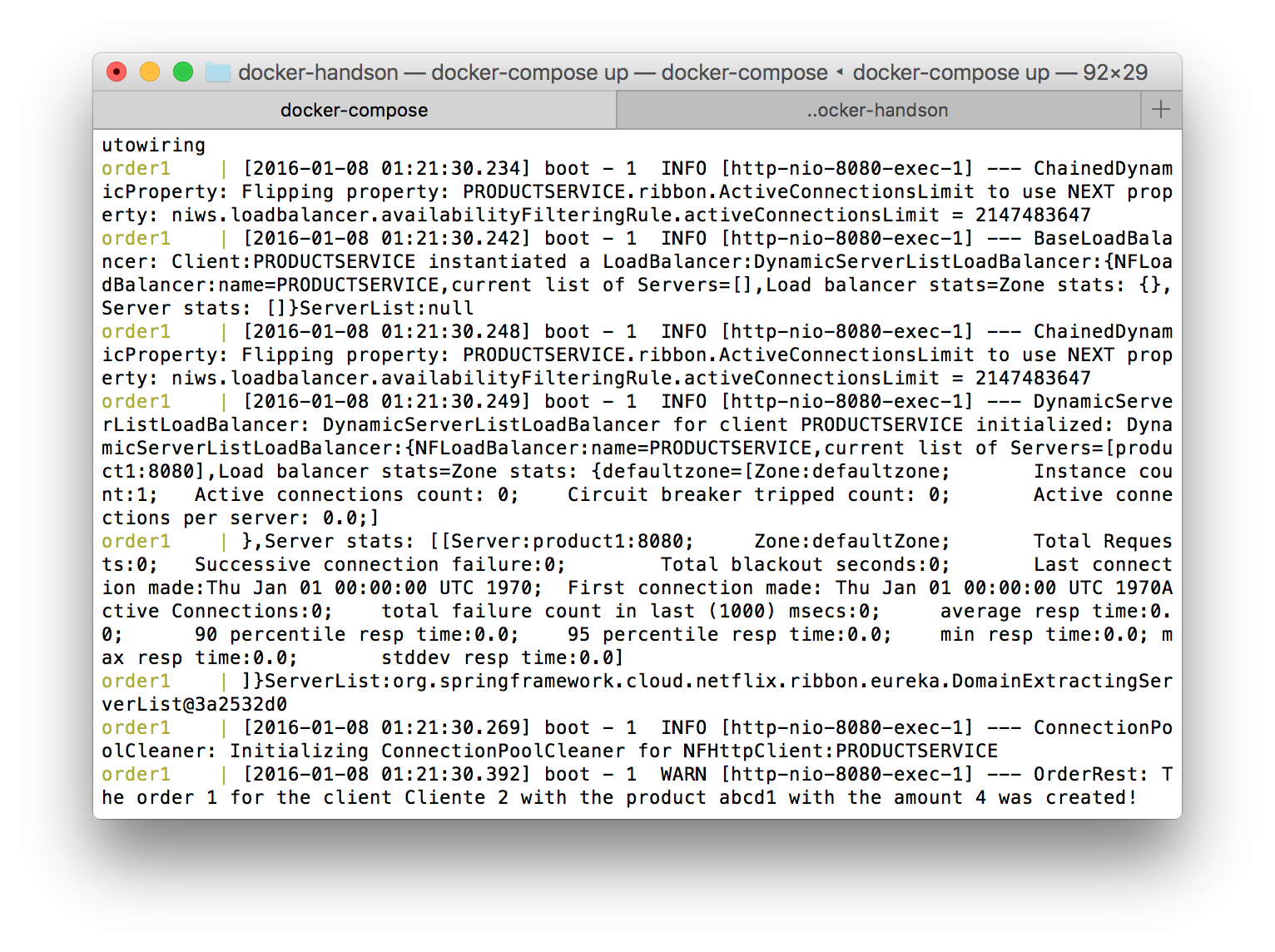
Success! But can we have further proof? If we see the logs from the Order1 container, we can see some logs showing Ribbon in action, searching for the services we need on the call and initializing load balancers, in order to serve our needs:

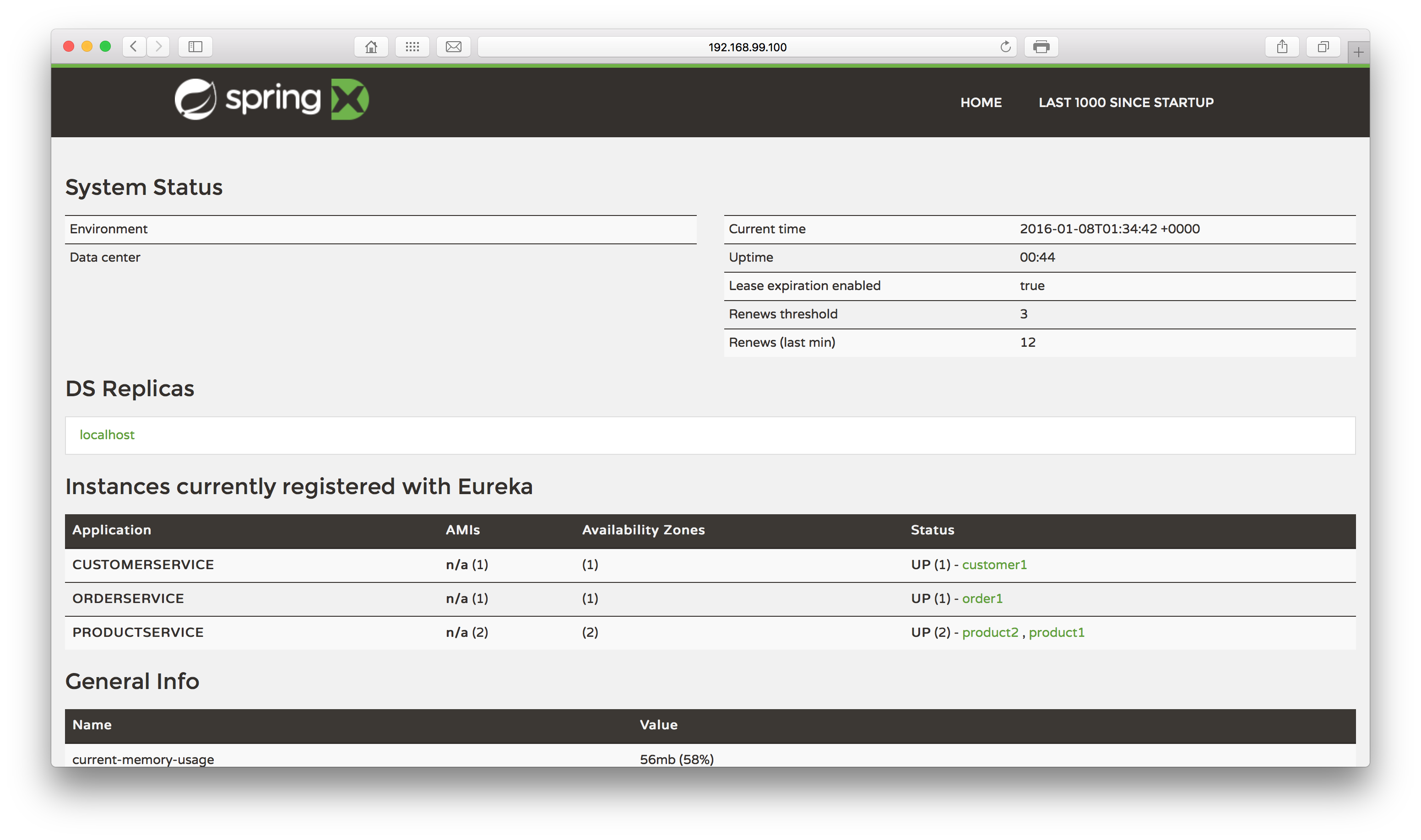
Let’s make one last test before closing in: let’s add one more instance of the Product’s service, to see if the new instance is registered under the same application ID. To do this, let’s run the following command. Notice that we didn’t specify the port to expose the service, since we just want to add up the instance to load balance the internal calls from the Order service:

docker run --rm --name product2 --hostname=product2 --net=microservicesnet -v /Users/alexandrelourenco/Applications/git/docker-handson:/data alexandreesl/microservices-spring-boot-base -jar /data/Product-backend/target/Product-backend-1.0.jar

If we open the Eureka web interface again, we will see that the second address is mapped:

Finally, to test the balance, let’s make a call of the previous URL of the Order service. After the call, we will see that our service is aware of both addresses, proving that the balance is implemented, as we can see on the log’s fragment bellow:

[2016-01-08 14:14:09.703] boot – 1 INFO [http-nio-8080-exec-1] — ChainedDynamicProperty: Flipping property: PRODUCTSERVICE.ribbon.ActiveConnectionsLimit to use NEXT property: niws.loadbalancer.availabilityFilteringRule.activeConnectionsLimit = 2147483647

[2016-01-08 14:14:09.709] boot – 1 INFO [http-nio-8080-exec-1] — BaseLoadBalancer: Client:PRODUCTSERVICE instantiated a LoadBalancer:DynamicServerListLoadBalancer:{NFLoadBalancer:name=PRODUCTSERVICE,current list of Servers=[],Load balancer stats=Zone stats: {},Server stats: []}ServerList:null

[2016-01-08 14:14:09.714] boot – 1 INFO [http-nio-8080-exec-1] — ChainedDynamicProperty: Flipping property: PRODUCTSERVICE.ribbon.ActiveConnectionsLimit to use NEXT property: niws.loadbalancer.availabilityFilteringRule.activeConnectionsLimit = 2147483647

[2016-01-08 14:14:09.718] boot – 1 INFO [http-nio-8080-exec-1] — DynamicServerListLoadBalancer: DynamicServerListLoadBalancer for client PRODUCTSERVICE initialized: DynamicServerListLoadBalancer:{NFLoadBalancer:name=PRODUCTSERVICE,current list of Servers=[product1:8080, product2:8080],Load balancer stats=Zone stats: {defaultzone=[Zone:defaultzone; Instance count:2; Active connections count: 0; Circuit breaker tripped count: 0; Active connections per server: 0.0;]

},Server stats: [[Server:product2:8080; Zone:defaultZone; Total Requests:0; Successive connection failure:0; Total blackout seconds:0; Last connection made:Thu Jan 01 00:00:00 UTC 1970; First connection made: Thu Jan 01 00:00:00 UTC 1970; Active Connections:0; total failure count in last (1000) msecs:0; average resp time:0.0; 90 percentile resp time:0.0; 95 percentile resp time:0.0; min resp time:0.0; max resp time:0.0; stddev resp time:0.0]

, [Server:product1:8080; Zone:defaultZone; Total Requests:0; Successive connection failure:0; Total blackout seconds:0; Last connection made:Thu Jan 01 00:00:00 UTC 1970; First connection made: Thu Jan 01 00:00:00 UTC 1970; Active Connections:0; total failure count in last (1000) msecs:0; average resp time:0.0; 90 percentile resp time:0.0; 95 percentile resp time:0.0; min resp time:0.0; max resp time:0.0; stddev resp time:0.0]

]}ServerList:org.springframework.cloud.netflix.ribbon.eureka.DomainExtractingServerList@2561f098

[2016-01-08 14:14:09.738] boot – 1 INFO [http-nio-8080-exec-1] — ConnectionPoolCleaner: Initializing ConnectionPoolCleaner for NFHttpClient:PRODUCTSERVICE

And that concludes our lab. As we can see, we builded a robust stack to deploy our microservices with their dependencies, with little effort.

Clustering container hosts

In all of our examples, we are always working with a single Docker host, our own machine on the case. On a real production environment, we can have some dozens or even hundreds of Docker hosts. In order to make all the hosts to work together, it is necessary to implement some layer that manages the hosts, making them appear as a single cluster to the consumers.

This is the goal of Docker Swarm. With Docker Swarm, we can connect multiple Docker hosts across a network, using them as a single cluster by using Docker Swarm’s interface.

For further information about Docker Swarm alongside a good example of utilization, I suggest consulting the excellent “The Docker Book”, which I describe on the next section.

References

This post was inspired by my studies on Docker with The Docker Book, written by James Turnbull. It is a excellent source of information, that I highly recommend to buy it! You can find the book available to purchase online on:

www.dockerbook.com

Conclusion

And this concludes our tour on the world of Docker. With a simple interface, Docker allows us to use all the power of the container world, allowing us to quickly deploy and escalate our applications. Never it was so simple to deploy our applications! Thank you for following me on another post, until next time.

ELK: using a centralized logging architecture – final part

Welcome, dear reader! This is the last part of our series about the ELK stack, that provides a centralized architecture for gathering and analyse of application logs. On this last part, we will see how we can construct a rich front-end for our logging solution, using Kibana.

Kibana

Also developed by Elasticsearch, Kibana provides a way to explore the data and/or build rich dashboards of our data on the indexer. With a simple configuration, that consist of pointing Kibana to a ElasticSearch’s index – it also allows to point to multiple indexes at once, using a wildcard configuration -, it allow us to quickly set up a front-end for our stack.

So, without further delay, let’s begin our last step on the setup of our solution.

Hands-on

Installation

Beginning our lab, let’s download Kibana from the site. To do this, let’s open a terminal and type the following command:

curl https://download.elasticsearch.org/kibana/kibana/kibana-4.0.0-linux-x64.tar.gz | tar -zx

PS: this lab assumes the reader is using a linux 64-bit OS (I am using Ubuntu 14.10). If the reader is using another type of OS, the download page for Kibana is the following:

http://www.elasticsearch.org/overview/kibana/installation/

After running the command, we can see a folder called “kibana-4.0.0-linux-x64”. That’s all we need to do to install Kibana on our lab. Before we start running, however, we need to start both Logstash and ElasticSearch, to make our whole stack go live. If the reader didn’t have the stack set up, please refer to part 1 and part 2.

One configuration that the reader may take note is the elasticsearch_url property, inside the “kibana.yml” file, on the config folder. Since we didn’t change the default port from our elasticsearch’s cluster and we are running all the tools on the same machine, there is no need to change anything, but on a real world scenario, you may need to change this property to point to your elasticsearch’s cluster. The reader can made other configurations as well on this file, such as configuring a SSL connection between Kibana and Elasticsearch or configure the name of the index Kibana will use to store his metadata on elasticsearch.

After we start the rest of the stack, it is time to run Kibana.To run it, we navigate to the bin folder of Kibana’s installation folder, and type:

./kibana

After some seconds, we can see that Kibana has successfully booted:

Set up

Now, let’s start using Kibana. Let’s open a web browser and enter:

http://localhost:5601/

On our first run, we will be greeted with the following screen:

The reason because we are seeing this screen is because we dont have any index configured. It is on this screen that we can, for example, point to multiple indexes. If we think, for example, about the default naming pattern of logstash’s plugin, we can see that, for each new date we run, logstash will demand the creation of a new index with the pattern “logstash-%{+YYYY.MM.dd}”. So, if we want Kibana to use all the indexes created this way on a single dataset, we simply configure the field with the value “logstash-*”

On our case, we change the default naming of the index, to demonstrate the possible configurations of the tool, so we change the field to “log4jlogs”. One important thing to note on logstash’s plugin documentation, is that the idea behind the index pattern is to make more easy to do operations such as deleting old data, so in a real world scenario, it would be more wise to leave the default pattern enabled.

The other field we need to set is the Time-field name . This field is used by Kibana as a primary filter, allowing him to filter the data from the dashboards and data explorations on a timeline perspective. If we see our document type from the documents storing log information on elasticsearch, we can see it has a field called @timestamp. This field is perfectly fit to our time-field need, so we put “@timestamp” in the field.

After we click on the “create” button, we will be sent to a new page, where we can see all the fields from the index we pointed, proving that our configuration was a success:

Of course, there is other settings as well that we can configure, such as the precision on the numeric fields or the date mask when showing this kind of data on the interface, all available on the “advanced” menu. For our lab needs, however, the default options will suffice, so we leave this page by clicking on the “Discover” menu.

Discovering the data

When we enter the new page, if we didnt send any data to the cluster in the last 15 minutes, we will see a message of no data found (see bellow). The reason for this is because, by default, Kibana limits the results for the last 15 minutes only. To change this, we can either change the time limit by clicking on the value on the upper right corner of the page, or by running again the java program from the previous post, so we have more fresh data.

After we set some data to explore, we can see that the page changes to a data view, where we can dinamically change field filters, by changing the left menu, and drill down the data to the fields level, as we can see bellow. The reader can feel free to explore the page before we move on to our next part.

Dashboards

Now that we have all set, let’s begin by creating a simple dashboard. we will create a pie chart of the messages by the log level, a table view showing the count of messages by class and a line chart of the error messages across the time.

First, let’s begin with the pie chart. We will select, from the menu, “Visualize” , then follow this sequence of options on the next pages:

pie chart >> from a new search

We will enter a page like the one bellow:

In this page, we will make our log level pie chart. To do this, we leave the metrics area unchanged, with the “count” value as slice size. Then, we choose “split slices” on the buckets area and select a “terms” aggregation, by the field “priority”. The screen bellow show our pie chart born!

After we made our chart, before we leave this page, we click on the disk icon on the top menu, input a name for our chart – also called visualization by Kibana’s terminology – and save it, for later use.

Now it is time for our table view. From the same menu we used to save our pie chart, click on the most left icon, called “new visualization”, then select “data table” and “from a new search”. We will see a similar page from the pie chart one, with similar options of aggregations and metrics to configure. With the intent of not bothering the reader with much repetitive instructions, from now on I will keep the explanation the more graphical possible, by the screenshots.

So, our data table view is made by making the configurations we can see on the left menu:

Analogous with what we made on the previous visualization, let’s also save the table view and click on new visualization, selecting line chart this time. The configuration for this chart can be seen bellow:

That concludes our visualizations. Now, let’s conclude our lab by making a dashboard that will show all the visualizations we build on the same page. To do this, first we select the “dashboard” option on the top menu. We will be greeted with the screen bellow:

This is the dashboard page, where we can create, edit and load dashboards. To add visualizations, we simply click on the plus icon on the top right side and select the visualization we want to add, like we can see bellow:

After we add the visualizations, it is pretty simple to arrange them: all we have to do is to drag and drop the visualizations as we like. My final arrangement of the dashboard is bellow, but the reader can arrange the way he finds best:

Finally, to save the dashboard, we simply click on the disk icon and input a name for our dashboard.

Cons

Of course, we cant make a complete overview of a tool, if we dont mention any noticeable con of it. The most visible downside of Kibana, on my opinion, is the lack of a native support to authentication and authorization. The reader may notice, by our tour of the interface, that there is no user or permission CRUDs whatsoever. Indeed, Kibana doesnt come with this feature.

One common workaround for this is to configure basic authentication on the web server Kibana runs with it – if we were using Kibana 3 on our lab, we would have to install manually a web server and deploy Kibana on it. On Kibana 4, we dont have to do this, because Kibana comes with a embedded node.js – , so the authentication is made by URL patterns. This link to the official node.js documentation provides a path to set basic authentication on the embedded server Kibana comes with it. The file that starts the server and need to be edited is on /src/bin/kibana.js.

Very recently, Elasticsearch has released shield, a plugin that implements a versatile security layer on Elasticsearch and subsequently on Kibana. Evidently, is a much more elegant and complete solution then the previous one, but the reader has to keep it in mind that he has to acquire a license to use shield.

Conclusion

And that concludes our tour by the ELK stack. Of course, on a real world scenario, we have some more steps to do, like the aforementioned authentication configuration, the configuration of purge policies and so on.However, we still can see that the core features we need were implemented, with very little effort. Like we talked about on the beginning of our series, logging information is a very rich source of information, that it has to be better explored on the business world. Thanks to everyone that follows my blog, until next time.

ELK: using a centralized logging architecture – part 2

Welcome, dear reader, to another post of our series about the ELK stack for logging. On the last post, we talked about LogStash, a tool that allow us to integrate data from different sources to different destinations, using transformations along the way, in a stream-like form. On this post, we will talk about ElasticSearch, a indexer based on apache Lucene, which can allow us to organize our data and make textual searches on the data, in a scalable infrastructure. So, let’s begin by understanding how ElasticSearch is organized on the inside

Indexes, documents and shards

On ElasticSearch, we have the concept of indexes. A index is like a repository, where we can store our data in the format of documents. A document on ElasticSearch’s terminology consists of a structure for the data to be stored, analysed and classified, following a mapping definition, composed of a series of fields – a important thing to note, is that a field on ElasticSearch has the same type across the whole index, meaning that we cant have a field “phone” with the type int on a document and the type string on another.

In turn, we have our documents stored on shards, which divide the data on segments based on a rule – by default, the segmentation is made by hashing the data, but it can also be manually manipulated -, making the searches faster.

So, in a nutshell, we can say that the order of organization of ElasticSearch is as follows:

Index >> Document (mappings/type) >> shard

This organization is used by the user on the two basic operations of the cluster: indexing and searching.

One last thing to say about documents is that they can not only be stored as independent , but also be mounted on a tree-like hierarchy, with links between them. This is useful in scenarios that we can make use of hierarchical searches, such as product’s searches based on their categories.

Indexing

Indexing is the action of inputing the data from a external source to the cluster. ElasticSearch is a textual indexer, which means he can only analyse text on plain format, despite that we can use the cluster to store data in base64 format, using a plugin. Later on the post, we will see a example installation of a plugin, which are extensions we can aggregate to expand our cluster usability.

When we index our data, we define which fields are to be analysed, which analyser to use, if the default ones does not suffice and which fields we want to store the data on the cluster, so we can use as the result of our searches. One important thing to note about the indexing operations is that, despite it has CRUD-like operations, the data is not really updated or deleted on the cluster, instead a new version is generated and the old version is marked as deleted.

This is a important thing to take note, because if not properly configured to make purges – which can be made with a configuration that break the shards into segments, and periodically make merges of the segments, phisically deleting the obsolet documents on the process -, the cluster will keep indefinitely expanding in size with the “deleted” older versions of our data, making specially the searches to became really slow.

All the operations can be made with a REST API provided by ElasticSearch, that we will see later on this post.

Searching

The other, and probably most important, action on ElasticSearch, is the searching of the data previously indexed. Like the indexing action, ElasticSearch also provide a REST API for the searches. The API provides a very rich range of possibilities of searching, from basic term searches to more complex searches such as hierarchical searches, searches by synonims, language detections, etc.

All the searching is based on a score system, where formulas are applied to confront the accuracy of the documents founded versus the query supplied. This score system can also be customized.

By default, the searching on the cluster occurs in 2 phases:

On the first phase, the master node sends the query for all the nodes, and subsequently shards , retrieving just the IDs and scores of the documents. Using a parameter called size which defines the maximum results from a query, the master selects the more meaningful documents, based on the score;
On the second phase, the master send requests for the nodes to retrieve the documents selected on the previous phase. After receiving the documents, the master finally sends the result for the client;

Alongside this search type, there’s also other modes, like the query_and_fetch. On this mode, the searching is made simultaneous on all shards, not only to retrieve the IDs and scores but also returning the data itself, limited only by the size parameter, which is applied per shard. In turn, on this mode, the maximum of results returned will be the size parameter plus the number of shards.

One interesting feature of ElasticSearch’s configuration options is the ability to make some nodes exclusive to query operations, and others to make the storage part, called data nodes. This way, when we query, our query dont need to run across all the cluster to formulate the results, making the searches faster. On the next section we will see a little more about cluster configurations.

Cluster capabilities

When we talk about a cluster, we talk about scalability, but we also talk about availability. On ElasticSearch, we can configure the replication of shards, where the data is replicated by a given factor, so we dont lose our data if a node is lost. The replication if also maintained by the cluster, so if we lost a replica, the cluster itself will distribute a new replica for another node.

Other interesting feature of the cluster are the ability to discover itself. By the default configuration, when we start a node he will use a discovery mode called Zen, which uses unicast and multicast to search for another instances on all the ports of the OS. If it founds another instance, and the name of the cluster is the same – this is another one of the cluster’s configuration properties. All of this configurations can be made on the file elasticsearch.yml, on the config folder -, it will communicate with the instance and establish a new node for the already running cluster. There is another modes for this feature, including the discover of nodes from other servers.

Logging

The reader could be thinking: “Lol, do I need all of this to run a logging stack?”.

Of course that ElasticSearch is a very robust tool, that can be used on other solutions as well. However, on our case of making a centralized logging analysis solution, the core of ElasticSearch’s capabilities serve us well for this task, after all, we are talking about the textual analysis of log texts, for use on dashboards, reports, or simply for real-time exploration of the data.

Well, that concludes the conceptual part of our post. Now, let’s move on to the practice.

Hands-on

So, without further delay, let’s begin the hands-on. For this, we will use the previous Java program we used on our lab about LogStash. The code can be found on GitHub, on this link. On this program, we used the org.apache.log4j.net.SocketAppender from log4j to send all the logging we make to LogStash. However, on that point we just printed the messages on the console, instead of sending to ElasticSearch. Before we change this, let’s first start our cluster.

To do this, first we need to download the last version from the site and unzip the tar. Let’s open a terminal, and type the following command:

curl https://download.elasticsearch.org/elasticsearch/elasticsearch/elasticsearch-1.4.4.tar.gz | tar -zx

After running the command, we will find a new folder called “elasticsearch-1.4.4” created on the same folder we run our command. To our example, we will create 2 copies of this folder on a folder we call “elasticsearchcluster”, where each one will represent one node of the cluster. To do this, we run the following commands:

mkdir elasticsearchcluster

sudo cp -avr elasticsearch-1.4.4/ elasticsearchcluster/elasticsearch-1.4.4-node1/

sudo cp -avr elasticsearch-1.4.4/ elasticsearchcluster/elasticsearch-1.4.4-node2/

After we made our cluster structure, we dont need the original folder anymore, so we remove:

rm -R elasticsearch-1.4.4/

Now, let’s finally start our cluster! To do this, we open a terminal, navigate to the bin folder of our first node (elasticsearch-1.4.4-node1) and type:

./elasticsearch

After some seconds, we can see our first node is on:

For curiosity sake, we can see the name “Feral” on the node’s name on the log. All the names generated by the tool are based on Marvel Comic’s characters. IT world sure has some sense of humor, heh?

Now, let’s start our second node. On a new terminal window, let’s navigate to the folder of our second node (elasticsearch-1.4.4-node2) and type again the command “./elasticsearch”. After some seconds, we can see that the node is also started:

One interesting thing to notice is that our second node “Ooze”, has a mention of comunicating with our other node, “Feral”. That is the zen discover on the action, making the 2 nodes talk to each other and form a cluster. If we look again at the terminal of our first node, we can see another evidence of this bidirectional communication, as “Feral” has added “Ooze” to the cluster, as his role as a master node:

Now that we have our cluster set up, let’s adjust our logstash script to send the messages to the cluster. To do this, let’s change the output part of the script, to the following:

input {
log4j {
port => 1500
type => “log4j”
tags => [ “technical”, “log”]
}
}

output {
stdout { codec => rubydebug }
elasticsearch_http {
host => “localhost”
port => 9200
index => “log4jlogs”
}
}

As we can see, we just included another output – we remained the console output just to check how logstash is receiving the data – including the ip and port where our ElasticSearch cluster will respond. We also defined the name of the index we want our logs to be stored. If this parameter is not defined, logstash will order elasticsearch to create a index with the pattern “logstash-%{+YYYY.MM.dd}”.

To execute this script, we do like we did on the previous post, we put the new script on a file called “configelasticsearch.conf” on the bin folder of logstash, and run with the command:

./logstash -f configelasticsearch.conf

PS1: On the GitHub repository, it is possible to find this config file, alongside a file containing all the commands we will send to ElasticSearch from now on.

PS2: For simplicity sake, we will use the default mappings logstash provide for us when sending messages to the cluster. It is also possible to pass a elasticsearch’s mapping structure, which consists of a JSON model, that logstash will use as a template. We will see the mapping from our log messages later on our lab, but for satisfying the reader curiosity for now, this is what a elasticsearch’s mapping structure look like, for example for a document type “product”:

“mappings” : {
“product”: {
“properties” : {

“variation” : { “type” : int }

“color” : { “type” : “string” }

“code” : { “type” : int }

“quantity” : { “type” : int }

}
}
}

After some seconds, we can see that LogStash booted, so our configuration was a success. Now, let’s begin sending our logs!

To do this, we run the program from our previous post, running the class com.technology.alexandreesl.LogStashProvider . We can see on the console of logstash, after starting the program, that the messages are going through the stack:

Now that we have our cluster up and running, let’s start to use it. First, let’s see the mappings of the index that ElasticSearch created for us, based on the configuration we made on LogStash. Let’s open a terminal and run the following command:

curl -XGET ‘localhost:9200/log4jlogs/_mapping?pretty’

On the command above, we are using ElasticSearch’s REST API. The reader will notice that, after the ip and port, the URL contains the name of the index we configured. This pattern for calls of the API is applied to most of the actions, as we can see below:

So, after this explanation, let’s see the result from our call:

{
“log4jlogs” : {
“mappings” : {
“log4j” : {
“properties” : {
“@timestamp” : {
“type” : “date”,
“format” : “dateOptionalTime”
},
“@version” : {
“type” : “string”
},
“class” : {
“type” : “string”
},
“file” : {
“type” : “string”
},
“host” : {
“type” : “string”
},
“logger_name” : {
“type” : “string”
},
“message” : {
“type” : “string”
},
“method” : {
“type” : “string”
},
“path” : {
“type” : “string”
},
“priority” : {
“type” : “string”
},
“stack_trace” : {
“type” : “string”
},
“tags” : {
“type” : “string”
},
“thread” : {
“type” : “string”
},
“type” : {
“type” : “string”
}
}
}
}
}
}

As we can see, the index “log4jlogs” was created, alongside the document type “log4j”. Also, a series of fields were created, representing information from the log messages, like the thread that generated the log, the class, the log level and the log message itself.

Now, let’s begin to make some searches.

Let’s begin by searching all log messages which the priority was “INFO”. We make this searching by running:
curl -XGET ‘localhost:9200/log4jlogs/log4j/_search?q=priority:info&pretty=true’
A fragment of the result of the query would be something like the following:

{
“took” : 12,
“timed_out” : false,
“_shards” : {
“total” : 5,
“successful” : 5,
“failed” : 0
},
“hits” : {
“total” : 18,
“max_score” : 1.1823215,
“hits” : [ {
“_index” : “log4jlogs”,
“_type” : “log4j”,
“_id” : “AUuxkDTk8qbJts0_16ph”,
“_score” : 1.1823215,
“_source”:{“message”:”STARTING DATA COLLECTION”,”@version”:”1″,”@timestamp”:”2015-02-22T13:53:12.907Z”,”type”:”log4j”,”tags”:[“technical”,”log”],”host”:”127.0.0.1:32942″,”path”:”com.technology.alexandreesl.LogStashProvider”,”priority”:”INFO”,”logger_name”:”com.technology.alexandreesl.LogStashProvider”,”thread”:”main”,”class”:”com.technology.alexandreesl.LogStashProvider”,”file”:”LogStashProvider.java:20″,”method”:”main”}
}

.

.

.

As we can see, the result is a JSON structure, with the documents that met our search. The beginning information of the result is not the documents themselves, but instead information about the search itself, such as the number of shards used, the seconds the search took to execute, etc. This kind of information is useful when we need to make a tuning of our searches, like manually defining the shards we which to use on the search, for example.

Let’s see another example. On our previous search, we received all the fields from the document on the result, which is not always the desired result, since we will not always use the whole information. To limit the fields we want to receive, we make our query like the following:
curl -XGET ‘localhost:9200/log4jlogs/log4j/_search?pretty=true’ -d ‘
{
“fields” : [ “priority”, “message”,”class” ],
“query” : {
“query_string” : { “query” : “priority:info” }
}
}’
On the query above, we asked ElasticSearch to limit the return to only return the priority, message and class fields. A fragment of the result can be seen bellow:

.

.

.

{
“_index” : “log4jlogs”,
“_type” : “log4j”,
“_id” : “AUuxkECZ8qbJts0_16pr”,
“_score” : 1.1823215,
“fields” : {
“priority” : [ “INFO” ],
“message” : [ “CLEANING UP!” ],
“class” : [ “com.technology.alexandreesl.LogStashProvider” ]
}
}

.

.

.

Now, let’s use the term search. On the term searches, we use ElasticSearch’s textual analysis to find a term inside the text of a field. Let’s run the following command:
curl -XGET ‘localhost:9200/log4jlogs/log4j/_search?pretty=true’ -d ‘
{
“fields” : [ “priority”, “message”,”class” ],
“query” : {
“term” : {
“message” : “up”
}
}
}’
If we see the result, it would be all the log messages that contains the word “up”. A fragment of the result can be seen bellow:

{
“_index” : “log4jlogs”,
“_type” : “log4j”,
“_id” : “AUuxkESc8qbJts0_16pv”,
“_score” : 1.1545612,
“fields” : {
“priority” : [ “INFO” ],
“message” : [ “CLEANING UP!” ],
“class” : [ “com.technology.alexandreesl.LogStashProvider” ]
}
}

Of course, there is a lot more of searching options on ElasticSearch, but the examples provided on this post are enough to make a good starting point for the reader. To make a final example, we will use the “prefix” search. On this type of search, ElasticSearch will search for terms that start with our given text, on a given field. For example, to search for log messages that have words starting with “clea”, part of the word “cleaning”, we run the following:
curl -XGET ‘localhost:9200/log4jlogs/log4j/_search?pretty=true’ -d ‘
{
“fields” : [ “priority”, “message”,”class” ],
“query” : {
“prefix” : {
“message” : “clea”
}
}
}’
If we see the results, we will see that are the same from the previous search, proving that our search worked correctly.

Kopf

The reader possibly could ask “Is there another way to send my queries without using the terminal?” or “Is there any graphical tool that I can use to monitor the status of my cluster?”. As a matter of fact, there is a answer for both of this questions, and the answer is the kopf plugin.

As we said before, plugins are extensions that we can install to improve the capacities of our cluster. In order to install the plugin, first let’s stop both the nodes of the cluster – press ctrl+c on both terminal windows to stop – then, navigate to the nodes root folder and type the following:

bin/plugin -install lmenezes/elasticsearch-kopf

If the plugin was installed correctly, we should see a message like the one bellow on the console:

.

.

.

-> Installing lmenezes/elasticsearch-kopf…
Trying https://github.com/lmenezes/elasticsearch-kopf/archive/master.zip…
Downloading …………………………………………………………………………………………………………………………………………………………………………………………………………………………………………………………………………………………………………………………………………………………………………………………………………………………………………………………………………………………………………………………………..DONE
Installed lmenezes/elasticsearch-kopf into….

After installing on both nodes, we can start again the nodes, just as we did before. After the booting of the cluster, let’s open a browser and type the following URL:

http://localhost:9200/_plugin/kopf

We will see the following web page of the kopf plugin, showing the status of our cluster, such as the nodes, the indexes, shard information, etc

Now, let’s run our last example from the search queries on kopf. First, we select the “rest” option on the top menu. On the next screen, we select “POST” as the http method, include on the URL field the index and document type to narrow the results and on the textarea bellow we include our JSON query filters. The print bellow shows the query made on the interface:

Conclusion

And so we conclude our post about ElasticSearch. A very powerful tool on the indexing and analysis of textual information, the central stone on our ELK stack for logging is a tool to be used, not only on a logging analysis system, but on other solutions that his features can be useful as well.

So, our stack is almost complete. We can gather our log information, and the information is indexed on our cluster. However, a final piece remains: we need a place where we can have a more friendly interface, that allow us not only to search the information, but also to make rich presentations of the data, such as dashboards. That’s when it enters our last part of our ELK series and the last tool we will see, Kibana. Thank you for following me on another post, until next time.

ELK: using a centralized logging architecture – part 1

Welcome, dear reader, to another post from my blog. On this new series, we will talk about a architecture specially designed to process data from log files coming from applications, with the junction of 3 tools, Logstash, ElasticSearch and Kibana. But after all, do we really need such a structure to process log files?

Stacks of log

On a company ecosystem, there is lots of systems, like the CRM, ERP, etc. On such environments, it is common for the systems to produce tons of logs, which provide not only a real-time analysis of the technical status of the software, but could also provide some business information too, like a log of a customer’s behavior on a shopping cart, for example. To dive into this useful source of information, enters the ELK architecture, which name came from the initials of the software involved: ElasticSearch, LogStash and Kibana. The picture below shows in a macro vision the flow between the tools:

As we can see, there’s a clear separation of concerns between the tools, where which one has his own individual part on the processing of the log data:

Logstash: Responsible for collect the data, make transformations like parsing – using regular expressions – adding fields, formatting as structures like JSON, etc and finally sending the data to various destinations, like a ElasticSearch cluster. Later on this post we will see more detail about this useful tool;
ElasticSearch: RESTful data indexer, ElasticSearch provides a clustered solution to make searches and analysis on a set of data. On the second part of our series, we will see more about this tool;
Kibana: Web-based application, responsible for providing a light and easy-to-use dashboard tool. On the third and last part of our series, we will see more of this tool;

So, to begin our road in the ELK stack, let’s begin by talking about the tool responsible for integrating our data: LogStash.

LogStash installation

To install, all we need to do is unzip the file we get from LogStash’s site and run the binaries on the bin folder. The only pre-requisite for the tool is to have Java installed and configured in the environment. If the reader wants to follow my instructions with the same system then me, I am using Ubuntu 14.10 with Java 8, which can be downloaded from Oracle’s site here.

With Java installed and configured, we begin by downloading and unziping the file. To do this, we open a terminal and input:

curl https://download.elasticsearch.org/logstash/logstash/logstash-1.4.2.tar.gz | tar xz

After the download, we will have LogStash on a folder on the same place we run our ‘curl’ command. On the LogStash terminology, we have 4 types of configurations we can make for a stream, named:

input: On this configuration, we put the sources of our streams, that can range from polling files of a file system to more complex inputs such as a Amazon SQS queue and even Twitter;
codec: On this configuration we make transformations on the data, like turning into a JSON structure, or grouping together lines that are semantically related, like for example, a Java’s stack trace;
filter: On this configuration we make operations such as parsing data from/to different formats, removal of special characters and checksums for deduplication;
output: On this configuration we define the destinations for the processed data, such as a ElasticSearch cluster, AWS SQS, Nagios etc;

Now that we have established LogStash’s configuration structure, let’s begin with our first execution. In LogStash we have two ways to configure our execution, one way by providing the settings on the start command itself and the other one is by providing a configuration file for the command. The simplest way to boot a LogStash’s stream is by setting the input and output as the console itself, to make this execution, we open a terminal, navigate to the bin folder of our LogStash’s installation and execute the following command:

./logstash -e ‘input { stdin { } } output { stdout {} }’

As we can see after we run the command, we booted LogStash, setting the console as the input and the output, without any transformation or filtering. To test, we simply input anything on the console, seeing that our message is displayed back by the tool:

Now that we get the installation out of the way, let’s begin with the actual lab. Unfortunately -or not, depending on the point of view -, it would take us a lot of time to show all the features of what we can do with the tool, so to make a short but illustrative example, we will start 2 logstash streams, to do the following:

1st stream:

The input will be made by a java program, which will produce a log file with log4j, representing technical information;
For now, we will just print logstash’s events on the console, using the rubydebug codec. On our next part on the series, we will return to this configuration and change the output to send the events to elasticsearch;

2nd stream:

The input will be made by the same java program, which will produce a positional file, representing business information of costumers and orders;
We will then use the grok filter to parse the data of the positional file into separated fields, producing the data for the output step;
Finally, we use the mongodb output, to save our data – filtering to only persist the orders – on a Mongodb collection;

With the streams defined, we can begin our coding. First, let’s create the java program which will generate the inputs for the streams. The code for the program can be seen bellow:

package com.technology.alexandreesl;

import java.io.FileWriter;
import java.io.IOException;
import java.io.PrintWriter;
import java.util.ArrayList;
import java.util.Date;
import java.util.List;

import org.apache.log4j.Logger;

public class LogStashProvider {

private static Logger logger = Logger.getLogger(LogStashProvider.class);

public static void main(String[] args) throws IOException {

try {

logger.info(“STARTING DATA COLLECTION”);

List<String> data = new ArrayList<String>();

Customer customer = new Customer();
customer.setName(“Alexandre”);
customer.setAge(32);
customer.setSex(‘M’);
customer.setIdentification(“4434554567”);

List<Order> orders = new ArrayList<Order>();

for (int counter = 1; counter < 10; counter++) {

Order order = new Order();

order.setOrderId(counter);
order.setProductId(counter);
order.setCustomerId(customer.getIdentification());
order.setQuantity(counter);

orders.add(order);

}

logger.info(“FETCHING RESULTS INTO DESTINATION”);

PrintWriter file = new PrintWriter(new FileWriter(
“/home/alexandreesl/logstashdataexample/data”
+ new Date().getTime() + “.txt”));

file.println(“1” + customer.getName() + customer.getSex()
+ customer.getAge() + customer.getIdentification());

for (Order order : orders) {
file.println(“2” + order.getOrderId() + order.getCustomerId()
+ order.getProductId() + order.getQuantity());
}

logger.info(“CLEANING UP!”);

file.flush();
file.close();

// forcing a error to simulate stack traces
PrintWriter fileError = new PrintWriter(new FileWriter(
“/etc/nopermission.txt”));

} catch (Exception e) {

logger.error(“ERROR!”, e);
}

}

}

As we can see, it is a very simple class, that uses log4j to generate some log and output a positional file representing data from customers and orders and at the end, try to create a file on a folder we don’t have permission to write by default, “forcing” a error to produce a stack trace. The complete code for the program can be found here. Now that we have made our data generator, let’s begin the configuration for logstash. The configuration for our first example is the following:

input {
log4j {
port => 1500
type => “log4j”
tags => [ “technical”, “log”]
}
}

output {
stdout { codec => rubydebug }
}

To run the script, let’s create a file called “config1.conf” and save the file with the script on the “bin” folder of logstash’s installation folder. Finally, we run the script with the following command:

./logstash -f config1.conf

This will start logstash process with the configurations we provided. To test, simply run the java program we coded earlier and we will see a sequence of message events in logstash’s console window, generated by the rubydebug codec, like the one bellow, for example:

{
“message” => “ERROR!”,
“@version” => “1”,
“@timestamp” => “2015-01-24T19:08:10.872Z”,
“type” => “log4j”,
“tags” => [
[0] “technical”,
[1] “log”
],
“host” => “127.0.0.1:34412”,
“path” => “com.technology.alexandreesl.LogStashProvider”,
“priority” => “ERROR”,
“logger_name” => “com.technology.alexandreesl.LogStashProvider”,
“thread” => “main”,
“class” => “com.technology.alexandreesl.LogStashProvider”,
“file” => “LogStashProvider.java:70”,
“method” => “main”,
“stack_trace” => “java.io.FileNotFoundException: /etc/nopermission.txt (Permission denied)\n\tat java.io.FileOutputStream.open(Native Method)\n\tat java.io.FileOutputStream.<init>(FileOutputStream.java:213)\n\tat java.io.FileOutputStream.<init>(FileOutputStream.java:101)\n\tat java.io.FileWriter.<init>(FileWriter.java:63)\n\tat com.technology.alexandreesl.LogStashProvider.main(LogStashProvider.java:66)”
}

Now, let’s move on to the next stream. First, we create another file, called “config2.conf”, on the same folder we created the first one. On this new file, we create the following configuration:

input {
file {
path => “/home/alexandreesl/logstashdataexample/data*.txt”
start_position => “beginning”
}
}

filter {
grok {
match => [ “message” , “(?<file_type>.{1})(?<name>.{9})(?<sex>.{1})(?<age>.{2})(?<identification>.{10})” , “message” , “(?<file_type>.{1})(?<order_id>.{1})(?<costumer_id>.{10})(?<product_id>.{1})(?<quantity>.{1})” ]
}
}

output {
stdout { codec => rubydebug }
if [file_type] == “2” {
mongodb {
collection => “testData”
database => “mydb”
uri => “mongodb://localhost”
}
}
}

With the configuration created, we can run our second example. Before we do that, however, let’s dive a little on the configuration we just made. First, we used the file input, which will make logstash keep monitoring the files on the folder and processing them as they appear on the input folder.

Next, we create a filter with the grok plugin. This filter uses combinations of regular expressions, that parses the data from the input. The plugin comes with more then 100 patterns pre-made that helps the development. Another useful tool in the use of grok is a site where we could test our expressions before use. Both links are available on the links section at the end of this post.

Finally, we use the mongodb plugin, where we reference our logstash for a database and collection of a mongodb instance, where we will insert the data from the file into mongodb’s documents. We also used again the rubydebug codec, so we can also see the processing of the files on the console. The reader will note that we used a “if” statement before the configuration of the mongodb output. After we parse the data with grok, we can use the newly created fields to do some logic on our stream. In this case, we filter to only process data with the type “2”, so only the order’s data goes to the collection on mongodb, instead of all the data. We could have expanded more on this example, like saving the data into two different collections, but for the idea of passing a general view of the structure of logstash for the reader, the present logic will suffice.

PS: This example assumes the reader has mongodb installed and running on the default port of his environment, with a db “mydb” and a collection “testData” created. If the reader doesn’t have mongodb, the instructions can be found on the official documentation.

Finally, with everything installed and configured, we run the script, with the following command:

./logstash -f config2.conf

After logstash’s start, if we run our program to generate a file, we will see logstash working the data, like the screen bellow:

And finally, if we query the collection on mongodb, we see the data is persisted:

Conclusion

And so we conclude the first part of our series. With a simple usage, logstash prove to be a useful tool in the integration of information from different formats and sources, specially log-related. In the next part of our series, we will dive in the next tool of our stack: ElasticSearch. Until next time

Hands-on: Using Google API to make searches on your applications

Welcome, dear reader, to another post of my blog. On this post, we will learn to use Google’s custom search API. With this API, you can make searches using Google’s infrastructure, enriching searching business features, like a web crawler, for example.

Pre-steps

Before we start coding, we need to create the keys to make our authentication with the API. One key is the API key itself and the other one is the search engine key. A search engine key is a key to a search engine you create to pre-filter the types of domains you want to make for your searches, so you dont end up searching sites in chinese, for example, if your application only want sites from England.

To start, access the site https://console.developers.google.com. After inputting our credentials, we get to the main site, where we can create a project, activate/deactivate APIs and generate a API key for the project. This tutorial from Google explain how to create API keys.

After that, we need to create the search engine key, on the site https://www.google.com/cse/all. We can follow this tutorial from Google to create the key.

Hands-on

On this hands-on, we will use Eclipse Luna and Maven 3.2.1. First, create a Maven project, without a archetype:

After creating our project, we add the dependencies. Instead of offering a Java library for the consumption, Google’s API consists of a URL, which is called by a simple GET execution, and returns a JSON structure. For the return, we will use a JSON API we used on our previous post. First, we add the following dependencies in our pom.xml:

<dependencies>
<dependency>
<groupId>javax.json</groupId>
<artifactId>javax.json-api</artifactId>
<version>1.0</version>
</dependency>
<dependency>
<groupId>org.glassfish</groupId>
<artifactId>javax.json</artifactId>
<version>1.0.4</version>
</dependency>
<dependency>
<groupId>org.jsoup</groupId>
<artifactId>jsoup</artifactId>
<version>1.7.2</version>
</dependency>
</dependencies>

Finally, with the dependencies included, we write our code. In this example, we will make a call to the API for a search with the string “java+android”. The API has a limit usage of 100 results per search – in the free mode -, and uses a pagination format of 10 results per page, so we will make 10 calls to the API. The following code make our example:

package com.technology.alexandreesl;

import java.io.BufferedReader;
import java.io.InputStreamReader;
import java.io.StringReader;
import java.net.HttpURLConnection;
import java.net.URL;

import javax.json.Json;
import javax.json.stream.JsonParser;
import javax.json.stream.JsonParser.Event;

public class GoogleAPIJava {

final static String apiKey = “<insert your API Key here>”;
final static String customSearchEngineKey = “<insert your search engine key here>”;

// base url for the search query
final static String searchURL = “https://www.googleapis.com/customsearch/v1?”;

public static void main(String[] args) {

int inicio = 1;

int contador = 0;

while (contador < 10) {

System.out
.println(“***************** SEARCH **************************”);
System.out.println(“”);

String result = “”;

result = read(“java+android”, inicio, 10);

JsonParser parser = Json.createParser(new StringReader(result));

while (parser.hasNext()) {
Event event = parser.next();

if (event == Event.KEY_NAME) {

if (parser.getString().equals(“htmlTitle”)) {
Event value = parser.next();

if (value == Event.VALUE_STRING)
System.out.println(“Title (HTML): ”
+ parser.getString());
}

if (parser.getString().equals(“link”)) {

Event value = parser.next();

if (value == Event.VALUE_STRING)
System.out.println(“Link: ” + parser.getString());
}

}

}

inicio = inicio + 10;

contador++;

System.out
.println(“**************************************************”);

}

}

private static String read(String qSearch, int start, int numOfResults) {
try {

String toSearch = searchURL + “key=” + apiKey + “&cx=”
+ customSearchEngineKey + “&q=”;

toSearch += qSearch;

toSearch += “&alt=json”;

toSearch += “&start=” + start;

toSearch += “&num=” + numOfResults;

URL url = new URL(toSearch);
HttpURLConnection connection = (HttpURLConnection) url
.openConnection();
BufferedReader br = new BufferedReader(new InputStreamReader(
connection.getInputStream()));
String line;
StringBuffer buffer = new StringBuffer();
while ((line = br.readLine()) != null) {
buffer.append(line);
}
return buffer.toString();
} catch (Exception e) {
e.printStackTrace();
}
return null;
}

}

As we can see above, we make use of the java.net standard classes to make the calls. Using counters to control the calls for the API. The result when we run the program is a list of sites for the search string printed on the console:

***************** SEARCH **************************

Title (HTML): Java Manager; Emulate Java – Android Apps on Google Play
Link: https://play.google.com/store/apps/details?id=com.java.manager
Title (HTML): How do I get Java for Mobile device?
Link: https://www.java.com/en/download/faq/java_mobile.xml
Title (HTML): AIDE – Android IDE – Java, C++ – Android Apps on Google Play
Link: https://play.google.com/store/apps/details?id=com.aide.ui
Title (HTML): Como obtenho o Java para Dispositivos Móveis?
Link: https://www.java.com/pt_BR/download/faq/java_mobile.xml
Title (HTML): Download java for android tablet – Android – Android Smartphones
Link: http://www.tomsguide.com/forum/id-1608121/download-java-android-tablet.html
Title (HTML): java.lang | Android Developers
Link: http://developer.android.com/reference/java/lang/package-summary.html
Title (HTML): Comparison of Java and Android API – Wikipedia, the free …
Link: http://en.wikipedia.org/wiki/Comparison_of_Java_and_Android_API
Title (HTML): Learn Java for Android Development: Introduction to Java – Tuts+ …
Link: http://code.tutsplus.com/tutorials/learn-java-for-android-development-introduction-to-java–mobile-2604
Title (HTML): java.text | Android Developers
Link: http://developer.android.com/reference/java/text/package-summary.html
Title (HTML): Apostila Java – Desenvolvimento Mobile com Android | K19
Link: http://www.k19.com.br/downloads/apostilas/java/k19-k41-desenvolvimento-mobile-com-android
**************************************************
***************** SEARCH **************************

Title (HTML): How can I access a Java-based website on an Android phone?
Link: http://www.makeuseof.com/answers/access-javabased-website-android-phone/
Title (HTML): Introduction to Java Variables | Build a Simple Android App (retired …
Link: http://teamtreehouse.com/library/build-a-simple-android-app/getting-started-with-android/introduction-to-java-variables-2
Title (HTML): Java Basics for Android Development – Part 1 – Treehouse Blog
Link: http://blog.teamtreehouse.com/java-basics-for-android-development-part-1
Title (HTML): GC: android – GrepCode Java Project Source
Link: http://grepcode.com/project/repository.grepcode.com/java/ext/com.google.android/android
Title (HTML): Java Essentials for Android
Link: https://www.udemy.com/java-essentials-for-android/
Title (HTML): How to Get Java on Android: 10 Steps (with Pictures) – wikiHow
Link: http://www.wikihow.com/Get-Java-on-Android
Title (HTML): Learn Android 4.0 Programming in Java
Link: https://www.udemy.com/android-tutorial/
Title (HTML): Trending Java repositories on GitHub today · GitHub
Link: https://github.com/trending?l=java
Title (HTML): Developing for Android in Eclipse: R.java not generating – Stack …
Link: http://stackoverflow.com/questions/2757107/developing-for-android-in-eclipse-r-java-not-generating
Title (HTML): Cling – Java/Android UPnP library and tools
Link: http://4thline.org/projects/cling/
**************************************************
***************** SEARCH **************************

Title (HTML): Getting Started | Android Developers
Link: https://developer.android.com/training/
Title (HTML): Java API – Android | Vuforia Developer Portal
Link: https://developer.vuforia.com/resources/api/main
Title (HTML): Java Programming for Android Developers For Dummies: Burd …
Link: http://www.amazon.com/Java-Programming-Android-Developers-Dummies/dp/1118504380
Title (HTML): Android Quickstart – Firebase
Link: https://www.firebase.com/docs/android/quickstart.html
Title (HTML): Learn Java for Android Development: Jeff Friesen: 9781430264545 …
Link: http://www.amazon.com/Learn-Java-Android-Development-Friesen/dp/1430264543
Title (HTML): Unity – Manual: Building Plugins for Android
Link: http://docs.unity3d.com/Manual/PluginsForAndroid.html
Title (HTML): Eclipse, Android and Java training and support
Link: http://www.vogella.com/
Title (HTML): AIDE – Android Java IDE download – Baixaki
Link: http://www.baixaki.com.br/android/download/aide-android-java-ide.htm
Title (HTML): Java Multi-Platform and Android SDK | Philips Hue API
Link: http://www.developers.meethue.com/documentation/java-multi-platform-and-android-sdk
Title (HTML): Android Client Tutorial – Java — Google Cloud Platform
Link: https://cloud.google.com/appengine/docs/java/endpoints/getstarted/clients/android/
**************************************************
***************** SEARCH **************************

Title (HTML): Gradle Plugin User Guide – Android Tools Project Site
Link: http://tools.android.com/tech-docs/new-build-system/user-guide
Title (HTML): Where is a download for java for android tablet? – Download …
Link: http://www.tomshardware.com/forum/52818-34-where-download-java-android-tablet
Title (HTML): Download android java
Link: http://www.softonic.com.br/s/android-java
Title (HTML): Binding a Java Library | Xamarin
Link: http://developer.xamarin.com/guides/android/advanced_topics/java_integration_overview/binding_a_java_library_(.jar)/
Title (HTML): java-ide-droid – JavaIDEdroid allows you to create native Android …
Link: http://code.google.com/p/java-ide-droid/
Title (HTML): Code Style Guidelines for Contributors | Android Developers
Link: https://source.android.com/source/code-style.html
Title (HTML): Eclipse Downloads
Link: https://eclipse.org/downloads/
Title (HTML): Open source Java for Android? Don’t bet on it | InfoWorld
Link: http://www.infoworld.com/article/2615512/java/open-source-java-for-android–don-t-bet-on-it.html
Title (HTML): Make your First Android App! – YouTube
Link: http://www.youtube.com/watch?v=A_qaarY4_lY
Title (HTML): Runtime for Android apps – BlackBerry Developer
Link: http://developer.blackberry.com/android/
**************************************************
***************** SEARCH **************************

Title (HTML): Java Mobile Android Basic Course Online
Link: http://www.vtc.com/products/javamobileandroidbasic.htm
Title (HTML): Android Game Development Tutorial – Kilobolt
Link: http://www.kilobolt.com/game-development-tutorial.html
Title (HTML): Learn Java for Android Development, 3rd Edition – Free Download …
Link: http://feedproxy.google.com/~r/IT-eBooks/~3/oITagjK1kYU/
Title (HTML): Cursos de Android e iOS | Caelum
Link: http://www.caelum.com.br/cursos-mobile/
Title (HTML): Autobahn|Android Documentation — AutobahnAndroid 0.5.2 …
Link: http://ottogrib.appspot.com/autobahn.ws/android
Title (HTML): Dagger ‡ A fast dependency injector for Android and Java.
Link: http://google.github.com/dagger/
Title (HTML): Dagger
Link: http://square.github.com/dagger/
Title (HTML): Setup – google-api-java-client – Download and Setup Instructions …
Link: https://code.google.com/p/google-api-java-client/wiki/Setup
Title (HTML): How to Write a ‘Hello World!’ app for Android
Link: http://www.instructables.com/id/How-to-Write-a-Hello-World-app-for-Android/
Title (HTML): The real history of Java and Android, as told by Google | ZDNet
Link: http://www.zdnet.com/article/the-real-history-of-java-and-android-as-told-by-google/
**************************************************
***************** SEARCH **************************

Title (HTML): Microsoft Releases SignalR SDK for Android, Java — Visual Studio …
Link: http://visualstudiomagazine.com/articles/2014/03/07/signalr-sdk-for-android-and-java.aspx
Title (HTML): Android Game Tutorials | Java Code Geeks
Link: http://www.javacodegeeks.com/tutorials/android-tutorials/android-game-tutorials/
Title (HTML): libgdx
Link: http://libgdx.badlogicgames.com/
Title (HTML): Buck: An Android (and Java!) build tool
Link: https://www.diigo.com/04w2jy
Title (HTML): Google copied Java in Android, expert says | Computerworld
Link: http://www.computerworld.com/article/2512514/government-it/google-copied-java-in-android–expert-says.html
Title (HTML): Reinventing Mobile Development (mobile app development mobile …
Link: http://www.codenameone.com/
Title (HTML): Understanding R.java
Link: http://knowledgefolders.com/akc/display?url=DisplayNoteIMPURL&reportId=2883&ownerUserId=satya
Title (HTML): Download Java Programming for Android Developers For Dummies …
Link: http://kickasstorrentsproxy.com/java-programming-for-android-developers-for-dummies-epub-pdf-t8208814.html
Title (HTML): Court sides with Oracle over Android in Java patent appeal – CNET
Link: http://www.cnet.com/news/court-sides-with-oracle-over-android-in-java-patent-appeal/
Title (HTML): Google Play Android Developer API Client Library for Java – Google …
Link: https://developers.google.com/api-client-library/java/apis/androidpublisher/v1
**************************************************
***************** SEARCH **************************

Title (HTML): Tape – A collection of queue-related classes for Android and Java by …
Link: http://shahmehulv.appspot.com/square.github.io/tape/
Title (HTML): Android Platform Guide
Link: http://cordova.apache.org/docs/en/4.0.0/guide_platforms_android_index.md.html
Title (HTML): OrmLite – Lightweight Object Relational Mapping (ORM) Java Package
Link: http://ormlite.com/
Title (HTML): Android Ported to C# | Xamarin Blog
Link: http://blog.xamarin.com/android-in-c-sharp/
Title (HTML): Tutorials | AIDE – Android IDE
Link: https://www.android-ide.com/tutorials.html
Title (HTML): All Tutorials on Mkyong.com
Link: http://www.mkyong.com/all-tutorials-on-mkyong-com/
Title (HTML): Top 10 Android Apps and IDE for Java Coders and Programmers
Link: https://blog.idrsolutions.com/2014/12/android-apps-ide-for-java-coder-programmers/
Title (HTML): Java Android developer information, news, and how-to advice …
Link: http://www.javaworld.com/category/java-android-developer
Title (HTML): Google Android e Java Micro Edition (ME)
Link: http://www.guj.com.br/forums/show/14.java
Title (HTML): Java & Android Obfuscator | DashO
Link: http://www.preemptive.com/products/dasho/overview
**************************************************
***************** SEARCH **************************

Title (HTML): Using a Custom Set of Java Libraries In Your RAD Studio Android …
Link: http://docwiki.embarcadero.com/RADStudio/XE7/en/Using_a_Custom_Set_of_Java_Libraries_In_Your_RAD_Studio_Android_Apps
Title (HTML): 50. Android (DRD) – java – CERT Secure Coding Standards
Link: https://www.securecoding.cert.org/confluence/pages/viewpage.action?pageId=111509535
Title (HTML): Gameloft: Top Mobile Games for iOS, Android, Java & more
Link: http://www.gameloft.com/
Title (HTML): Android and Java Developers: We Have a SignalR SDK for You!
Link: http://msopentech.com/blog/2014/03/06/android-java-developers-signalr-sdk/
Title (HTML): Java Swing UI on iPad, iPhone and Android
Link: http://www.creamtec.com/products/ajaxswing/solutions/java_swing_ui_on_ipad.html
Title (HTML): TeenCoder Java Series: Computer Programming Courses for Teens!
Link: http://www.homeschoolprogramming.com/teencoder/teencoder_jv_series.php
Title (HTML): Mixpanel Java API Overview – Mixpanel | Mobile Analytics
Link: https://mixpanel.com/help/reference/java
Title (HTML): AN 233 Java D2xx for Android API User Manual – FTDI
Link: http://www.ftdichip.com/Documents/AppNotes/AN_233_Java_D2XX_for_Android_API_User_Manual.pdf
Title (HTML): Xtend – Modernized Java
Link: http://eclipse.org/xtend/
Title (HTML): ProGuard
Link: http://freecode.com/urls/9ab4c148025d25c6eccd84906efb2c05
**************************************************
***************** SEARCH **************************

Title (HTML): FOSS Patents: Oracle wins Android-Java copyright appeal: API code …
Link: http://www.fosspatents.com/2014/05/oracle-wins-android-java-copyright.html
Title (HTML): java android 4.1.1 free download
Link: http://en.softonic.com/s/java-android-4.1.1
Title (HTML): Four reasons to stick with Java, and four reasons to dump it …
Link: http://www.javaworld.com/article/2689406/java-platform/four-reasons-to-stick-with-java-and-four-reasons-to-dump-it.html
Title (HTML): Java Programming for Android Developers For Dummies Cheat Sheet
Link: http://www.dummies.com/how-to/content/java-programming-for-android-developers-for-dummie.html
Title (HTML): Twitter4J – A Java library for the Twitter API
Link: http://twitter4j.org/
Title (HTML): Ignite Realtime: Smack API
Link: http://www.igniterealtime.org/projects/smack/
Title (HTML): Java Programming for Android Developers For Dummies
Link: http://allmycode.com/Java4Android
Title (HTML): Oracle ADF Mobile
Link: http://www.oracle.com/technetwork/developer-tools/adf-mobile/overview/adfmobile-1917693.html
Title (HTML): Introduction of How Android Works for Java Programmers
Link: http://javarevisited.blogspot.com/2013/06/introduction-of-how-android-works-Java-programmers.html
Title (HTML): Download java emulator for Android | JavaEmulator.com
Link: http://www.javaemulator.com/android-java-emulator.html
**************************************************
***************** SEARCH **************************

Title (HTML): Google hauls Java-on-Android spat into US Supreme Court • The …
Link: http://go.theregister.com/feed/www.theregister.co.uk/2014/10/09/google_takes_javaonandroid_case_to_supreme_court/
Title (HTML): Android SDK for Realtime Apps
Link: http://www.pubnub.com/docs/java/android/android-sdk.html
Title (HTML): Como Obter o Java no Android: 4 Passos (com Imagens)
Link: http://pt.wikihow.com/Obter-o-Java-no-Android
Title (HTML): If Android is so hot, why has Java ME overtaken it?
Link: http://fortune.com/2012/01/01/if-android-is-so-hot-why-has-java-me-overtaken-it/
Title (HTML): Android tutorial
Link: http://www.tutorialspoint.com/android/
Title (HTML): What’s New in IntelliJ IDEA 14
Link: https://www.jetbrains.com/idea/whatsnew/
Title (HTML): Android OnClickListener Example | Examples Java Code Geeks
Link: http://examples.javacodegeeks.com/android/core/view/onclicklistener/android-onclicklistener-example/
Title (HTML): JTwitter – the Java library for the Twitter API : Winterwell Associates …
Link: http://www.winterwell.com/software/jtwitter.php
Title (HTML): RL SYSTEM – Cursos Online de Android, .NET, Java, PHP, ASP …
Link: http://www.rlsystem.com.br/
Title (HTML): samples/ApiDemos/src/com/example/android/apis/app …
Link: https://android.googlesource.com/platform/development/+/master/samples/ApiDemos/src/com/example/android/apis/app/FragmentRetainInstance.java
**************************************************

Conclusion

And so we concluded our hands-on. With a simple usage, Google’s custom search API offers a simple but powerful tool in the belt of every developer who need to use a search engine of the internet in his solutions. Thank you for reading, until next time.

Source-code (Github)

Hands-on: Implementing MicroServices with Spring Boot

Welcome, dear reader, to another post from my technology blog. In this post, we will talk about an interesting architectural model, the microservices architecture, in addition to studying one of the new features of Spring 4.0, Spring Boot. But after all, what are microservices?

Microservices

In the development of large systems, it is common to develop various components and libraries that implement various functions, ranging from implementing business requirements to technical tasks, such as an XML parser, for example. In these scenarios, several components are reused by different interfaces and / or systems. Imagine, for example, a component that implements a register of customers and we package this component in a java project, which generates a deliverable jar file.

In this scenario, we have several interfaces to use this component, such as web applications, mobile, EJBs, etc. In the traditional form of Java implementation, we would package this jar deploy in several other packages, such as EAR files, WAR files, etc. Imagine now that a problem in the customer code is found. In this scenario, we have a considerable operational maintenance work, since as well as the correction on the component, we would have to make the redeploy of all consumer applications due to the component to be packaged inside the other deployment packages.

In order to propose a solution to this issue, was born the microservices architecture model. In this architectural model, rather than packaging the components as jar files to be packaged into consumer systems, the components are independently exposed in the form of remote accessibility APIs, consumed using protocols such as HTTP, for example. The figure below illustrates this architecture:

An important point to note in the above explanations, is that although we are exemplifying the model using the Java world, the same principles can be applied to other technologies such as C #, etc.

Spring Boot

Among the new features in version 4.0 of the Spring Framework, a new project that has arisen is the Spring Boot.The goal of Spring Boot is to provide a way to provide Java applications quickly and simply, through an embedded server – by default it used an embedded version of Tomcat – thus eliminating the need of Java EE containers. With Spring Boot, we can expose components such as REST services independently, exactly as proposed in the microservices architecture, so that in any maintenance of the components, we no longer make the redeploy of all its consumers.

So without further delay, let’s begin our hands-on. For this lab, we will use the Eclipse Luna and Maven 3 .

To illustrate the concept of microservices, we will create 3 Maven projects in this hands-on: each of them will symbolize back-end functionality, ie reusable APIs, and one of them held a composition, that is, will be a consumer of the other 2. All the code that will be presented is available in the links section at the end of this post.

To begin, let’s create 3 simple Maven projects without defined archetype, and let’s call them Product-backend, Customer-backend and Order-backend. In the poms of the 3 projects, we will add the dependencies for the creation of our REST services and the startup of Spring Boot, as we can see below:

.

.

.

<parent>
<groupId>org.springframework.boot</groupId>
<artifactId>spring-boot-starter-parent</artifactId>
<version>1.2.0.RELEASE</version>
</parent>

<dependencies>
<dependency>
<groupId>org.springframework.boot</groupId>
<artifactId>spring-boot-starter-web</artifactId>
</dependency>

<dependency>
<groupId>org.springframework.boot</groupId>
<artifactId>spring-boot-starter-jersey</artifactId>
</dependency>
</dependencies>

.

.

.

With the dependencies established, we start the coding. The first class that we create, that we call Application, will be identical in all three projects, because it only works as an initiator to Spring Boot – as defined by the @SpringBootApplication annotation – starting a Spring context and the embedded server:

package br.com.alexandreesl.handson;

import org.springframework.boot.SpringApplication;
import org.springframework.boot.autoconfigure.SpringBootApplication;

@SpringBootApplication
public class Application {
public static void main(String[] args) {
SpringApplication.run(Aplication.class, args);
}
}

The next class we will see is the ApplicationConfig. In this class, which uses the @Configuration Spring annotation to indicate to the framework that it is a resource configuration class, we set the Jersey, which is our ResourceManager responsible for exposing REST services for application consumers.

In a real application, this class would be also creating datasources for access to databases and other resources, but in order to keep a hands-on simple enough to be able to focus on the Spring Boot, we will use mocks to represent the data access.

package br.com.alexandreesl.handson;

import javax.inject.Named;

import org.glassfish.jersey.server.ResourceConfig;
import org.springframework.context.annotation.Configuration;

@Configuration
public class ApplicationConfig {

@Named
static class JerseyConfig extends ResourceConfig {
public JerseyConfig() {
this.packages(“br.com.alexandreesl.handson.rest”);
}
}

}

The above class will be used identically in the projects relating to customers and products. For orders, however, since it will be a consumer of the other services, we will use this class with a slight difference, as we will also instantiate a RestTemplate. This class, one of the novelties in the Spring Framework, is a standardized and very simple interface that facilitates the consumption of REST services. The class to use in the Order-backend project can be seen below:

package br.com.alexandreesl.handson;

import javax.inject.Named;

import org.glassfish.jersey.server.ResourceConfig;
import org.springframework.context.annotation.Bean;
import org.springframework.context.annotation.Configuration;
import org.springframework.web.client.RestTemplate;

@Configuration
public class ApplicationConfig {

@Named
static class JerseyConfig extends ResourceConfig {
public JerseyConfig() {
this.packages(“br.com.alexandreesl.handson.rest”);
}
}

@Bean
public RestTemplate restTemplate() {
RestTemplate restTemplate = new RestTemplate();

return restTemplate;
}

}

Finally, we will start the implementation of the REST services themselves. In the project Customer-backend, we create a class of DTO and a REST service. The class, which is a customer, is a simple POJO, as seen below:

package br.com.alexandreesl.handson.rest;

public class Customer {

private long id;

private String name;

private String email;

public long getId() {
return id;
}

public void setId(long id) {
this.id = id;
}

public String getName() {
return name;
}

public void setName(String name) {
this.name = name;
}

public String getEmail() {
return email;
}

public void setEmail(String email) {
this.email = email;
}

}

The REST service, in turn, has only 2 capabilities, a search of all customers and other search that query a customer from your id:

package br.com.alexandreesl.handson.rest;

import java.util.ArrayList;
import java.util.List;

import javax.inject.Named;
import javax.ws.rs.GET;
import javax.ws.rs.Path;
import javax.ws.rs.Produces;
import javax.ws.rs.QueryParam;
import javax.ws.rs.core.MediaType;

@Named
@Path(“/”)
public class CustomerRest {

private static List<Customer> clients = new ArrayList<Customer>();

static {

Customer customer1 = new Customer();
customer1.setId(1);
customer1.setName(“Cliente 1”);
customer1.setEmail(“customer1@gmail.com”);

Customer customer2 = new Customer();
customer2.setId(2);
customer2.setName(“Cliente 2”);
customer2.setEmail(“customer2@gmail.com”);

Customer customer3 = new Customer();
customer3.setId(3);
customer3.setName(“Cliente 3”);
customer3.setEmail(“customer3@gmail.com”);

Customer customer4 = new Customer();
customer4.setId(4);
customer4.setName(“Cliente 4”);
customer4.setEmail(“customer4@gmail.com”);

Customer customer5 = new Customer();
customer5.setId(5);
customer5.setName(“Cliente 5”);
customer5.setEmail(“customer5@gmail.com”);

clients.add(customer1);
clients.add(customer2);
clients.add(customer3);
clients.add(customer4);
clients.add(customer5);

}

@GET
@Produces(MediaType.APPLICATION_JSON)
public List<Customer> getClientes() {
return clients;
}

@GET
@Path(“customer”)
@Produces(MediaType.APPLICATION_JSON)
public Customer getCliente(@QueryParam(“id”) long id) {

Customer cli = null;

for (Customer c : clients) {

if (c.getId() == id)
cli = c;

}

return cli;
}

}

And that concludes our REST service for searching the customers. For the products, analogous to the customers, we have to search all products or one product through one of his ids and finally we have the order service, which through a “submitOrder” method gets the data of a product and a customer – whose keys are passed as parameters to the method – and return a order header. The classes that make up our product service within its Product-backend project are the following:

package br.com.alexandreesl.handson.rest;

public class Product {

private long id;

private String sku;

private String description;

public long getId() {
return id;
}

public void setId(long id) {
this.id = id;
}

public String getSku() {
return sku;
}

public void setSku(String sku) {
this.sku = sku;
}

public String getDescription() {
return description;
}

public void setDescription(String description) {
this.description = description;
}

}

package br.com.alexandreesl.handson.rest;

import java.util.ArrayList;
import java.util.List;

import javax.inject.Named;
import javax.ws.rs.GET;
import javax.ws.rs.Path;
import javax.ws.rs.Produces;
import javax.ws.rs.QueryParam;
import javax.ws.rs.core.MediaType;

@Named
@Path(“/”)
public class ProductRest {

private static List<Product> products = new ArrayList<Product>();

static {

Product product1 = new Product();
product1.setId(1);
product1.setSku(“abcd1”);
product1.setDescription(“Produto1”);

Product product2 = new Product();
product2.setId(2);
product2.setSku(“abcd2”);
product2.setDescription(“Produto2”);

Product product3 = new Product();
product3.setId(3);
product3.setSku(“abcd3”);
product3.setDescription(“Produto3”);

Product product4 = new Product();
product4.setId(4);
product4.setSku(“abcd4”);
product4.setDescription(“Produto4”);

products.add(product1);
products.add(product2);
products.add(product3);
products.add(product4);

}

@GET
@Produces(MediaType.APPLICATION_JSON)
public List<Product> getProdutos() {
return products;
}

@GET
@Path(“product”)
@Produces(MediaType.APPLICATION_JSON)
public Product getProduto(@QueryParam(“id”) long id) {

Product prod = null;

for (Product p : products) {

if (p.getId() == id)
prod = p;

}

return prod;
}

}

Finally, the classes that make up our aforementioned order service in the Order-backend project are:

package br.com.alexandreesl.handson.rest;

import java.util.Date;

public class Order {

private long id;

private long amount;

private Date orderDate;

private Customer customer;

private Product product;

public long getId() {
return id;
}

public void setId(long id) {
this.id = id;
}

public long getAmount() {
return amount;
}

public void setAmount(long amount) {
this.amount = amount;
}

public Date getOrderDate() {
return orderDate;
}

public void setOrderDate(Date orderDate) {
this.orderDate = orderDate;
}

public Customer getCustomer() {
return customer;
}

public void setCustomer(Customer customer) {
this.customer = customer;
}

public Product getProduct() {
return product;
}

public void setProduct(Product product) {
this.product = product;
}

}

package br.com.alexandreesl.handson.rest;

import java.util.Date;

import javax.inject.Inject;
import javax.inject.Named;
import javax.ws.rs.GET;
import javax.ws.rs.Path;
import javax.ws.rs.Produces;
import javax.ws.rs.QueryParam;
import javax.ws.rs.core.MediaType;

import org.springframework.web.client.RestTemplate;

@Named
@Path(“/”)
public class OrderRest {

private static long id = 1;

@Inject
private RestTemplate restTemplate;

@GET
@Path(“order”)
@Produces(MediaType.APPLICATION_JSON)
public Order submitOrder(@QueryParam(“idCustomer”) long idCustomer,
@QueryParam(“idProduct”) long idProduct,
@QueryParam(“amount”) long amount) {

Order order = new Order();

Customer customer = restTemplate.getForObject(
“http://localhost:8081/customer?id={id}”, Customer.class,
idCustomer);

Product product = restTemplate.getForObject(
“http://localhost:8082/product?id={id}”, Product.class,
idProduct);

order.setCustomer(customer);
order.setProduct(product);
order.setId(id);
order.setAmount(amount);
order.setOrderDate(new Date());

id++;

return order;
}
}

The reader should note the use of the product and customer classes in our order service. Such classes, however, are not direct references of the classes implemented in the other projects, but classes “cloned” from the original, within the order project. This apparent duplication of code in the DTO classes, sure to be a negative aspect of the solution, which can be seen as similar as stub classes we see in JAX-WS clients, must be measured carefully as it can be considered a small price to pay, considering the problems we see if we make the coupling of the projects.

A half solution that can minimize this problem, is to create a aditional project for the domain classes, which would be imported by all other projects, as the domain classes must undergo much lower maintenance than functionality itself. I leave it to the readers to assess the best option, according to the characteristics of their projects.

Good, but after all this coding, lets get down to, which is to test our services!

To begin, let’s start our REST services. For this, we create run configurations in Eclipse – like the image below – where we will add a system property, which specify the port where the spring boot will start the process. In my environment, I started the customer service on port 8081, the products in 8082 and the orders on port 8083, but the reader is free to use the most appropriate ports for his environment. The property to be used to configure the port is:

-Dserver.port=8081

PS: If the reader change the ports, you must correct the ports of the calls in the order service code.

With properly configured run configurations, we will start processing and test some calls to our REST. Simply click on each run configuration created, one at a time, which will generate 3 different console windows running in the Eclipse console window. As we see below, when we started the projects, Spring Boot generates a boot log, where you can see the embedded tomcat and its associated resources, such as Jersey, being initialized:

After booting the services, we can run them through the browser in order to test our implementation. For example, to test the query of all customers, if we type in the browser the following URL:

http://localhost:8081/

Obteremos como retorno a seguinte estrutura JSON:

[{"id":1,"nome":"Cliente 1","email":"cliente1@gmail.com"},{"id":2,"nome":"Cliente 2","email":"cliente2@gmail.com"},{"id":3,"nome":"Cliente 3","email":"cliente3@gmail.com"},{"id":4,"nome":"Cliente 4","email":"cliente4@gmail.com"},{"id":5,"nome":"Cliente 5","email":"cliente5@gmail.com"}]

Consisting of all registered customers in our mocks structure, showing that our service is working properly. To test the method that returns one particular customer from a id, we can enter a URL like the one below:

http://localhost:8081/customer?id=3

That returns a JSON with the customer data:

{"id":3,"nome":"Cliente 3","email":"cliente3@gmail.com"}

Similarly, to test if the product service is functioning properly, please call the URL:

http://localhost:8082/

Which produces the following result in JSON:

[{"id":1,"sku":"abcd1","descricao":"Produto1"},{"id":2,"sku":"abcd2","descricao":"Produto2"},{"id":3,"sku":"abcd3","descricao":"Produto3"},{"id":4,"sku":"abcd4","descricao":"Produto4"}]

Finally, to test the functionality of the order service we make a call, which through, for example, we simulate a order in which a customer of ID 2 wants the product of ID 3, and the amount of 4:

http://localhost:8083/order?idCustomer=2&idProduct=3&amount=4

We produce the following JSON, representing the header of a order effected:

{"id":1,"amount":4,"orderDate":1419530726399,"customer":{"id":2,"name":"Cliente 2","email":"customer2@gmail.com"},"product":{"id":3,"sku":"abcd3","description":"Produto3"}}

At this point, the reader may notice a bug in our order service: subsequent calls will generate the same orders with the same IDs! This is due to our mock variable that generates the ids be declared as a global variable that is recreated every new instance of the class. As REST services have request scope, every request generates a new instance, which means that the variable is never incremented through the calls. One of the simplest ways of fixing this bug is declaring the variable as static, but before we do that, let’s take a moment to think like the fact that we have implemented our services as microservices – yes, they are microservices! – Can help us in our maintenance:

– If we were in a traditional implementation, each of these components would be a jar file encapsulated within a client application such as a web application (WAR);

– Thus, for fixing this bug, and correcting the order code, we would also redeploy the product code, the customer code and the web application itself! The advantages become even more apparent if we consider that the application would have many more features in addition to the problematic one, which would make the redeploy of all the others, causing a complete unavailability of our system during reimplantation;

So, having realized the advantages of our construction format, we will initiate the maintenance. During the procedure, we will make the stop and restart of our order service in order to demonstrate how microservices do not affect each other’s availability.

To begin our maintenance, we will terminate the Spring Boot process of our order service. To do this, we simply select the corresponding console window and terminate it. If we call the URL of the order service, we have the following error message, indicating the unavailability:

However, if we try to call the product and customer services, we see that both are operational, proving the independence thereof.

Then we make the maintenance, changing the variable to the static type:

.

.

.

private static long id = 1;

.

.

.

Finally, we make a restart of the order service, with the implemented correction. If we run several calls to the URL of the service, we see that the service is generating orders with different IDs, proving that the fix was a success:

{"id":9,"amount":4,"orderDate":1419531614702,"customer":{"id":2,"name":"Cliente 2","email":"customer2@gmail.com"},"product":{"id":3,"sku":"abcd3","description":"Produto3"}}

We realize, with this simple example, that the microservices architecture brought us a powerful solution: you can stop, correct / evolve and start new versions of the components, without thereby requiring the redeployment of the whole system and its totally unavailable. Not to mention, that since we are using standard protocols such as HTTP to communicate, we could even use other technologies, like C# for example, to make a web front-end to our system.

Going beyond

Recently, I published a new post about microservices, where I demonstrate a evolution of this example, using a service registry to implement service discovery. Please, check it out the post here, I hope the reader will found very interesting!

Conclusion

And so we conclude our hands-on. With a simple but powerful implementation, Spring Boot is a good option to implement a microservices architecture that must be evaluated throughout every Java architect or developer who wants to promote this model in his projects. Thanks to everyone who supported me in this hands-on, until next time.

Hands-on Angularjs: Building single-page applications with Javascript

Welcome to another post from my blog. In this post, we’ll talk about a web framework that has become popular in the construction of single-page web applications: Angularjs. But after all, what is a single-page application?

Single-page applications

Single-page applications, as the name implies, consist of applications where only a single “page” – or as we also call, HTML document – is submitted to the client, and after this initial load, only fragments of the page are reloaded, by Ajax requests, without ever making a full page reload. The main advantage we have in this web application model is that, due to minimizing the data traffic between the client and the server, it provides the user with a highly dynamic application, with low “latency” between user actions on the interface. A point of attention, however, is that in this application model, much of the “weight” of the application processing falls to the client side, then the device’s capabilities where the user is accessing the application can be a problem for the adoption of the model, especially if we are talking about applications accessed on mobile devices.

Developed by Google, Angularjs brought features that allow you to build in a well structured way applications in single-page model, through the use of javascript as an extension built on top of HTML pages. One of the advantages of the framework is that it integrates seamlessly into HTML, allowing the developer team to, for example, reuse the pages of a prototype made by a web designer.

Architecture

The framework architecture works with the concept of been a html extension of the page to which it is linked. As a javascript library, imported within the pages, which through the use of policies – kind of attributes that are embedded within their own html tags, usually with the prefix “NG” – performs the compilation of all the code belonging to the framework generating dynamic code – html, css and javascript – that the user use through his browser. For readers who are interested in knowing more deeply the architecture behind the framework, the presentation below speaks in detail about this topic:

AngularJS Architecture from Eyal Vardi

Layout

Although the framework has high flexibility in the construction of layouts due to the use of pure html, it lacks ready layout options, so to make the application with a more pleasant graphical interface, it enters the bootstrap, providing CSS styles – plus pre-build behavior in javacript and dynamic html – that enable an even richer layout for the application. At the end of this post, beyond the official angularjs site, you can also access the link to the official site of the bootstrap.

The MVC model

In the web world, is well known the pattern MVC (Model – View – Controller). In this pattern, we define that the web application is defined in 3 layers with different responsibilities:

View: In this layer, we have the code related to the presentation to the end user, with pages and rules related to navigation, such as control of the flags of a register in the “wizard” format, for example.

Controller: This layer is the code that bridges between the navigation and the source of application data, represented by the model layer. Processing and business rules typically belong to this layer.

Model: In this layer is the code responsible for performing the persistence of the application data. In a traditional web application, we commonly have a DBMS as a data source.

Speaking in the context of angularjs, as we see below, we have the view layer represented by the html pages. These pages communicate with the controller layer through policies explained in the beginning of our post, invoking the controllers of the framework, consisting of a series of javascript functions encoded by the developer. These functions use a binding layer, provided by the framework, called $ scope, which is populated by the controller and displayed by the view, representing the model layer. Typically, in the architecture of a angularjs system, we have the model layer being filled through REST services.

The figure below illustrates the interaction between these layers:

Hands-on

For this hands-on, we will use the Wildfly 8.1.0 server, angularjs and the bootstrap. At the time of this post, the latest version (stable) of angularjs is 1.2.26 and for the bootstrap is 3.2.0. As IDE, I am using Eclipse Luna.

First, the reader must create a project of type “Dynamic Web Project” by selecting the wizard image below. In fact, it would be perfectly possible to use static web project as a project, but we’ll use the dynamic only to facilitate the deploy on the server.

Following the wizard, remember to select the runtime Wildfly, as indicated below, and select the checkbox that calls for the creation of the descriptor “web.xml” on the last page of the wizard.

At the end, we will have a project structure like the one below:

As a last step of project configuration, we will add the project in the automatically deployed application list on our Wildfly server. To do this, select the server from the perspective of servers, select the “add or remove” and move the application to the list of configured applications, as follows:

Including the angularjs and bootstrap on the application

To include the angular and the bootstrap in our application, simply include the contents thereof, consisting of js files, css, etc inside the folder “webcontent” generating the project structure below:

PS: This structure aims only to provide a quick and easy way to set the environment for the realization of our learning. In a real application, the developer has the freedom to not include all angular files, including only those whose resources will be used in the project.

Starting our development, we will create a simple page containing a single page application that consists of a list of tasks, with the option of new tasks and filtering tasks already completed. Keep in mind that the goal of this small application is only to show the basic structure of angularjs. In a real application, the js code should be structured in directories, ensuring readability and maintainability of the code.

Thus, we come to the implementation. To deploy it, we will create an html page called “index.html”, and put the code below:

<!DOCTYPE html>
<html ng-app=”todoApp”>
<head>
<title>Tarefas</title>
<link href=”css/bootstrap.css” rel=”stylesheet” />
<link href=”css/bootstrap-theme.css” rel=”stylesheet” />
<script src=”angular.js”></script>

<script>
var model = {
user: “Alexandre”,
items: [{ action: “Ir á padaria”, done: false },
{ action: “Comprar remédios”, done: false },
{ action: “Pagar contas”, done: true },
{ action: “Ligar para Ana”, done: false }]
};

var todoApp = angular.module(“todoApp”, []);

todoApp.filter(“checkedItems”, function () {
return function (items, showComplete) {
var resultArr = [];
angular.forEach(items, function (item) {

if (item.done == false || showComplete == true) {
resultArr.push(item);
}
});
return resultArr;
}
});

todoApp.controller(“ToDoCtrl”, function ($scope) {
$scope.todo = model;

$scope.addNewItem = function(actionText) {
$scope.todo.items.push({ action: actionText, done: false});
}

});
</script>

</head>
<body ng-controller=”ToDoCtrl”>
<div class=”page-header”>
<h1>
Tarefas de {{todo.user}}
</h1>
</div>
<div class=”panel”>
<div class=”input-group”>
<input class=”form-control” ng-model=”actionText” />

<button class=”btn btn-default”
ng-click=”addNewItem(actionText)”>Add</button>

</div>

<table class=”table table-striped”>
<thead>
<tr>
<th>Description</th>
<th>Done</th>
</tr>
</thead>
<tbody>
<tr ng-repeat=
“item in todo.items | checkedItems:showComplete | orderBy:’action'”>
<td>{{item.action}}</td>
<td><input type=”checkbox” ng-model=”item.done” /></td>
</tr>
</tbody>
</table>

<div class=”checkbox-inline”>
<label><input type=”checkbox” ng_model=”showComplete”> Show Complete</label>
</div>
</div>

</body>
</html>

As we can see, we have a simple html page. First, insert the policy “ng-app”, which initializes the framework on the page, and import the files needed for the operation of the angular and the bootstrap:

<html ng-app=”todoApp”>
<head>
<title>Tarefas</title>
<link href=”css/bootstrap.css” rel=”stylesheet” />
<link href=”css/bootstrap-theme.css” rel=”stylesheet” />
<script src=”angular.js”></script>

Following is the creation of a module. A angularjs module consists of other components such as filters and controllers, constituting a unit similar to a package that can be imported into other application modules. For the initial data source, we put a JSON structure in a JavaScript variable, which is inserted into the binding layer later. In addition, we also have to create a filter. Filters, as the name implies, are created to provide a means of filtering the data of a listing. Later on we will see that use in practice:

<script>
var model = {
user: “Alexandre”,
items: [{ action: “Ir á padaria”, done: false },
{ action: “Comprar remédios”, done: false },
{ action: “Pagar contas”, done: true },
{ action: “Ligar para Ana”, done: false }]
};

var todoApp = angular.module(“todoApp”, []);

todoApp.filter(“checkedItems”, function () {
return function (items, showComplete) {
var resultArr = [];
angular.forEach(items, function (item) {

if (item.done == false || showComplete == true) {
resultArr.push(item);
}
});
return resultArr;
}
});

Moving on we have the construction of the controller, which as already explained, is responsible for performing the interaction with the binding layer, beyond the call to external resources to the page, such as REST services. In our example, we link the JSON structure created earlier with our binding layer and create a function for adding new tasks to a action:

todoApp.controller(“ToDoCtrl”, function ($scope) {
$scope.todo = model;

$scope.addNewItem = function(actionText) {
$scope.todo.items.push({ action: actionText, done: false});
}

});
</script>

Once we have our populated binding, it is easy for us to display its values, as in the example below, where we show the value of “user”. We also define a form to our inclusion of tasks:

<body ng-controller=”ToDoCtrl”>
<div class=”page-header”>
<h1>
Tarefas de {{todo.user}}
</h1>
</div>
<div class=”panel”>
<div class=”input-group”>
<input class=”form-control” ng-model=”actionText” />

<button class=”btn btn-default”
ng-click=”addNewItem(actionText)”>Add</button>

</div>

Finally, we have the proper view of the tasks. To do this, we use the “ng-repeat” policy. The reader will notice that we have made use of our filter, and we ask the angularjs to order our list by the “action” value. In addition, we can also see the binding for changing the filter, through the checkboxes to enable / disable filtering, in addition to the marking of completed tasks

<table class=”table table-striped”>
<thead>
<tr>
<th>Description</th>
<th>Done</th>
</tr>
</thead>
<tbody>
<tr ng-repeat=
“item in todo.items | checkedItems:showComplete | orderBy:’action'”>
<td>{{item.action}}</td>
<td><input type=”checkbox” ng-model=”item.done” /></td>
</tr>
</tbody>
</table>

<div class=”checkbox-inline”>
<label><input type=”checkbox” ng_model=”showComplete”> Show Complete</label>
</div>
</div>

The final screen in operation can be seen below:

Conclusion

And so we conclude our post on angularjs. With design flexibility and an easy learning structure, its adoption as well as the single page applications model is a powerful tool that every web developer should have in his pocket knife options. Thanks to everyone who supported me in this post, until next time.

Technology explained

Technology blog from Alexandre Eleutério Santos Lourenço.

Web

gRPC: Transporting massive data with Google’s serialization

The escalation of data transfer

RPC

gRPC

Protocol Buffers

Types of gRPC applications

Synch vs. Asynch

Deadlines & timeouts

RPC termination

Channels

Tutorial

Set up

Creating the gRPC Service definition

Generating gRPC code

Building the server

Constructing the client

Making the call

Using streams

Running gRPC on Docker

Conclusion

Curator: Implementing purge routines on your Elasticsearch cluster

Elastalert: implementing rich monitoring with Elasticsearch

Docker: using containers to implement a Microservices architecture

ELK: using a centralized logging architecture – final part

ELK: using a centralized logging architecture – part 2

ELK: using a centralized logging architecture – part 1

Hands-on: Using Google API to make searches on your applications

Hands-on: Implementing MicroServices with Spring Boot

Hands-on Angularjs: Building single-page applications with Javascript