Hi, dear readers! Welcome to my blog. On this post, we will learn about Apache Kafka, a distributed messaging system which is being used on lots of streaming solutions.
This article will be divided on several sections, allowing the reader to not only understand the concepts behind but also a lab to exercise the concepts in practice. So, without further delay, let’s begin!
Kafka architecture
Overview
Kafka is a distributed messaging system created by Linkedin. On Kafka, we have stream data structures called topics, which can be consumed by several clients, organized on consumer groups. This topics are stored on a Kafka cluster, where which node is called a broker.
Kafka’s ecosystem also need a Zookeeper cluster in order to run. Zookeeper is a key-value storage solution, which on Kafka’s context is used to store metadata. Several operations such as topic creation are done on Zookeeper, instead of in the brokers.
The main difference from Kafka to other messaging solutions that utilizes classic topic structures is that on Kafka we have offsets. Offsets act like cursors, pointing to the last location a consumer and/or producer has reached consuming/producing messages for a given topic on a given partition.
Partitions on Kafka are like shards on some NOSQL databases: they divide the data, organizing by partition and/or message keys (more about this when we talk about ingesting data on Kafka).
So, on Kafka, we have producers ingesting data, controlled by producer offsets, while we have consumers consuming data from topics, also with their offsets. The main advantages on this approach are:
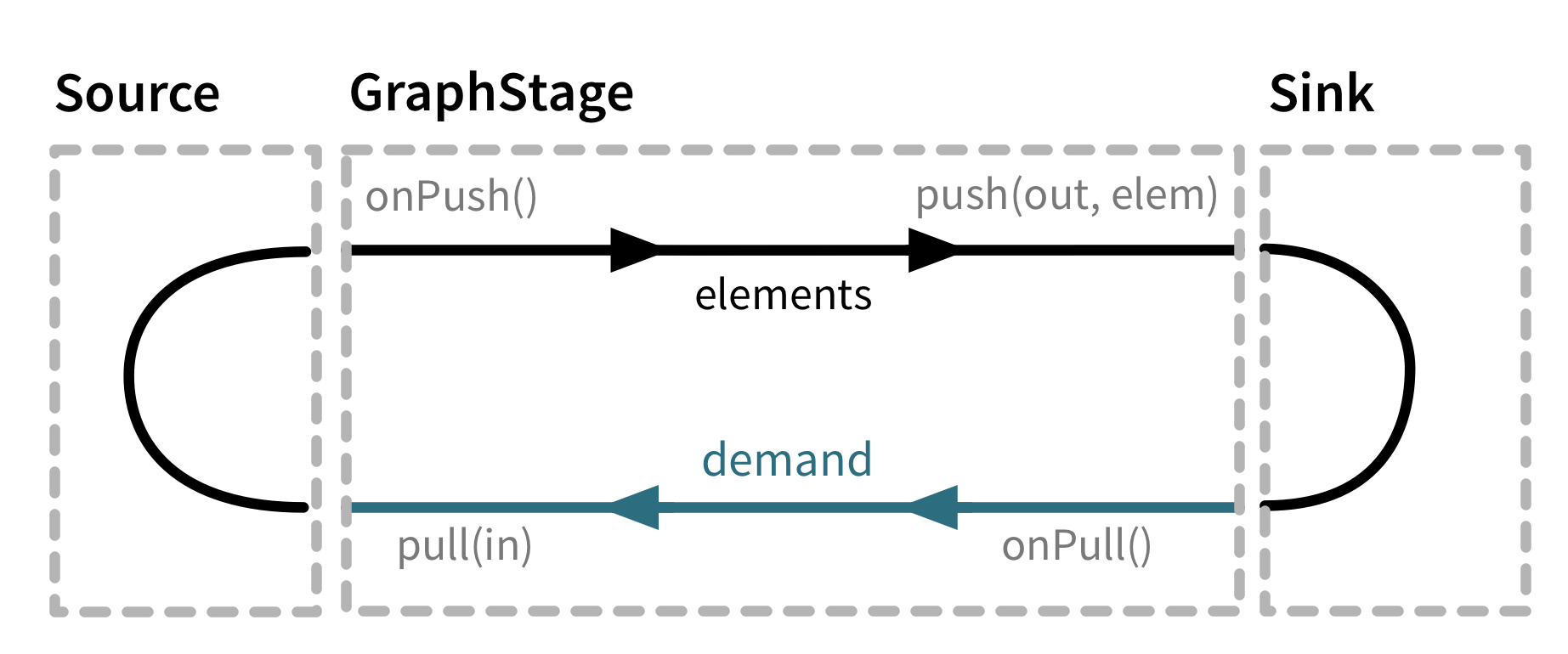
- Data can be read and replayed by consumers, since there’s no link between consumed data and produced data. This also allows to implement solutions with back-pressure, that is, solutions where consumers can poll data according to their processing limits;
- Data can be retained for more time, since on streams, different from classic topics, data is not removed from the structure after been sent to all consumers. It is also possible to compress the data on the stream, allowing Kafka clusters to retain lots of data on their streams;
Kafka’s offsets explained
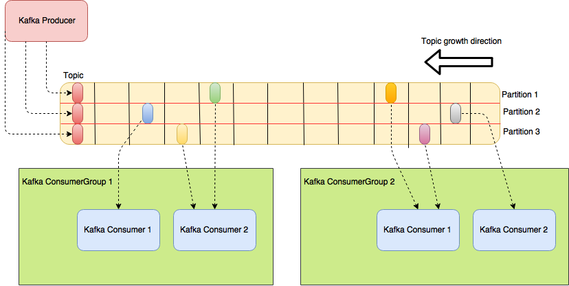
The following diagram illustrates a Kafka topic on the run:

Kafka Topic producer/consumer offsets
On the diagram, we can see a topic with 2 partitions. Each little rectangle represents a offset pointing to a location on the topic. On the producer side, we can see 2 offsets pointing to the topic’s head, showing our producer ingesting data on topic.
On Kafka, each partition is assigned to a broker and each broker is responsible for delivering production/consumption for that partition. The broker responsible for this is called a partition leader on Kafka.
How many partitions are needed for a topic? The main factor for this point is the desired throughput for production/consumption. Several factors are key for the throughput, such as the producer ack type, number of replicas etc.
Too much partitions are also something to take care when planning a new topic, as too much partitions can hinder availability and end-to-end latency, alongside memory consumption on the client side – remember that both producer and consumer can operate with several partitions at the same time. This article is a excellent reference for this matter.
On the consumer side, we see some interesting features. Each consumer has his own offset, consuming data from just one partition. This is a important concept on Kafka: each consumer is responsible for consuming one partition on Kafka and each consumer group consumes the data individually, that is, there is no relation between the consumption of one group and the others.
We can see this on the diagram, where the offsets from one group are on different positions from the others. All Kafka offsets are stored on a internal topic inside Kafka’s cluster, both producer and consumer offsets. Offsets are committed (updated) on the cluster using auto-commit or by committing manually on code, analogous as relational database commits. We will see more about this when coding our own consumer.
What happens when there’s more partitions than consumers? When this happens, Kafka’s delivers data from more then one partition to the same consumer, as we can see bellow. It is important to note that it is possible to increase the number of consumers on a group, avoiding this situation altogether:
The same consumer consuming from more then one partition on Kafka
One important thing to notice is what happens on the opposite situation, when there is less partitions than consumers configured:

Idle consumers on Kafka
As we can see, on this case, we end up with idle consumers, that won’t process any messages until a new partition is created. This is important to keep in mind when setting a new consumer on Kafka, as increasing too much the number of consumers will just end up with idle resources not been used at all.
One of the key features on Kafka is that it guarantees message ordering. This ordering is done on the messages within the same partition, but not on the whole topic. That means that when we consume data from Kafka with our consumers, the data across the partitions is read on parallel, but data from the same partition is read with a single thread, guaranteeing the order.
IMPORTANT: As stated on Kafka’s documentation, it is not recommended to process data coming from Kafka in parallel, as it will scramble the messages order. The recommended way to scale the solution is by adding more partitions, as it will add more threads to process data on parallel, without losing the ordering inside the partitions.
Partitions on Kafka are always written on a single mount point on disk. They are written on files, that are splitted when they reach a certain amount of data, or a certain time period – 1GB or 1 week of data respectively by default, whatever it comes first – that are called log segments. The more recent log segment, that represents the data ingested up to the head of the stream is called active segment and it is never deleted. The older segments are removed from disk according to the retention policies configured.
Replicas
In order to guarantee data availability, Kafka works with replicas. When creating a topic, we define how much replicas we want to have for each partition on the topic. If we configure we want 3 replicas, for example, that means that for a topic with 2 partitions, we will have 6 replicas from that topic, plus the 2 active partitions.
Kafka replicates the data just like we would do by hand: brokers that are responsible for maintaining the replicas – called partition followers – will subscribe for the topic and keep reading data from the partition leader and writing to their replicas. Followers that have data up-to-date with the leader are called In-Synch replicas. Replicas can become out of synch for example due to network issues, that causes the synching process to be slow and lag behind the leader to a unacceptable point.
Rebalance
When a rebalance occurs, for example if a broker is down, all the writing/reading from partitions that broker was a partition leader are ceased. The cluster elects a new partition leader, from one of the IS (In-Synch) replicas, and so the writing/reading is resumed.
During this period, applications that were using the old leader to publish data will receive a specific error when trying to use the partition, indicating that a rebalance is occurring (unless we configure the producer to just deliver the messages without any acknowledgment, which we will see in more detail on the next sections). On the consumer side, it is possible to implement a rebalance listener, which can clean up the work for when the partition is available again.
It is important to notice that, as a broker is down, it could be possible that some messages won’t be committed, causing messages to be processed twice when the partition processing is resumed.
What happens if a broker is down and no IS replicas are available? That depends on what we configured on the cluster. If unclean election is disabled, then all processing is suspended on that partition, until the broker that was down comes back again. If unclean election is enabled, then one of the brokers that were a follower is elected as leader.
Off course, each option has his advantages: without unclean election, we can lose the partition in case we can’t restart the lost broker, but with unclean election, we risk losing some messages, since their offsets will be overwritten by the new leader, when new data arrives at the partition.
If the old leader comes back again, it will resume the partition’s processing as a new follower, and it will not insert the lost messages in case of a unclean election.
Kafka’s producer explained
On this section, we will learn the internals that compose a Kafka producer, responsible for sending messages to Kafka topics. When working with the producer, we create ProducerRecords, that we send to Kafka by using the producer.
Producer architecture
Kafka producer internal structure is divided as we can see on the following diagram:

Kafka Producer internal details
As we can see, there is a lot going on when producing messages to Kafka. First, as said before, we create a ProducerRecord, that consist of 3 sections:
- Partition Key: The partition key is a optional field. If it is passed, it indicates the partition that it must be sent the message too;
- Message Key: The message key is a required field. If no partition key is passed, the partitioner will use this field to determine on which partition it will send the message. Kafka guarantees that all messages for a same given message key will always be sent to the same partition – as long as the number of partitions on a topic stay the same;
- Value (payload): The value field is a required field and, as obvious, is the message itself that must be sended;
All the fields from the ProducerRecord must be serialized to byte arrays before sent to Kafka, so that’s exactly what is done by the Serializer at the first step of our sending – we will see later on our lab that we always define a serializer for our keys and value – , after that, the records are sent to the Partitioner, that determines the partition to send the message.
The Partitioner then send the message to bulk processes, running on different threads, that “stack” the messages until a threshold is reached – a certain number of bytes or a certain time without new messages, whatever it comes first – and finally, after the threshold is reached, the messages are sent to the Kafka broker.
Let’s keep in mind that, as we saw before, brokers are elected as partition leaders for partitions on topics, so when sending the messages, they are sent directly to the partition leader’s broker.
Acknowledgment types
Kafka’s producer works with 3 types of acks (acknowledgments) that a message has been successfully sent. The types are:
- ack=0: The producer just send the message and don’t wait for a confirmation, even from the partition leader. Of course, this is fastest option to deliver messages, but there is also risk of message loss;
- ack=1: The producer waits for the partition leader to reply that wrote the message before moving on. This option is more safe, however, there is also some degree of risk, since a partition leader can go down just after the acknowledgement without repassing the message to any replica;
- ack=all: The producer waits for the partition leader and all IS replicas to write before moving on. This option is naturally the safest of all, but there is also the disadvantage of possible performance issues, due to waiting for all network replication to occur before continuing. This aggravates when there is no IS replicas at the moment, as it will hold the production until at least one replica is made;
Which one to use? That depends on the characteristics of the solution we are working with. A ack=0 could be useful on a solution that works with lots of messages that are not critic in case of losses – monitoring events, for example, are short-lived information that could be lost at certain degree – unlike, for example, bank account transactions, where ack=all is a must, since message losses are unacceptable on this kind of application.
Producer configurations
There are several configurations that could be made on the producer. Here we have some of the more basic and interesting ones to know:
- bootstrap.servers: A list of Kafka brokers for the producer to communicate with. This list is updated automatically when brokers are added/removed from the cluster, but it is advised to set at least 2 brokers, as the producer won’t start if just one broker is set and the broker is down;
- key.serializer: The serializer that it will be used when transforming the keys to byte arrays. Of course, the serializer class will depend on the keys type been used;
- value.serializer: The serializer that it will be used to transform the message to a byte array. When using complex types such as Java objects, it is possible to use one of the several out-of-box serializers, or implement your own;
- acks: This is where we define the acknowledgement type, as we saw previously;
- batch.size: This is the amount of memory the bulk process will wait to stack it up until reached to send the message batches;
- linger.ms: The amount of time, in milliseconds, the producer will wait for new messages, before sending the messages it has buffered. Of course, if the batch.size is reached first, then the message batch is sent before reaching this threshold;
- max.in.flight.requests.per.connection: This parameters defines how many messages the producer will send before waiting for responses from Kafka (if ack is not set as 0, of course). As stated on Kafka’s documentation, this configuration must be set to 1 to guarantee the messages on Kafka will be written at the same order they are sent by the producer;
- client.id: This parameter can be set with any string value and identifies the producer on the Kafka cluster. It is used by the cluster to build metrics and logging;
- compression.type: This parameter define a compression to be used on messages, before they are sent to Kafka. It supports snappy, gzip and lz4 formats. By default, no compression is used;
- retries: This parameter defines how many times the producer will retry sending a message to a broker, before notifying the application that a error has occurred;
- retry.backoff.ms: This parameter defines how many milliseconds the producer will wait between the retries. By default, the time is 100ms;
Kafka’s consumer explained
On this section, we will learn the internals that compose a Kafka consumer, responsible for reading messages from Kafka topics.
Consumer architecture
Kafka consumer internal structure is divided as we can see on the following diagram:

Kafka consumer internal details
When we request a Kafka broker to create a consumer group for one or more topics, the broker creates a Consumer Group Coordinator. Each broker has a group coordinator for the partitions it is the partition leader.
This component is responsible for deciding which consumer will be responsible for consuming which partitions, by the rules we talked about on the offsets section. It is also responsible for checking consumers health, by establishing heartbeat frequencies to be sent at intervals. If a consumer fails to send heartbeats, it is considered unhealthy, so Kafka delegates the partitions assigned to that consumer to another one.
The consumer, on his turn, uses a deserializer to convert the messages from byte arrays to the required types. Like with the producer, we can also use several different types of out-of-box deserializers, as well as creating our own.
IMPORTANT: Kafka consumer must always run on the main thread. If you try to create a consumer and delegate to run on another thread, there’s a check on the consumer that will thrown a error. This is due to Kafka consumer not been thread safe. The recommended way to scale a application that consumes from Kafka is by creating new application instances, each one running his own consumer on the same consumer group.
One important point to take note is that, when a message is delivered to Kafka, it only becomes available to consume after it is properly replicated to all IS replicas for his respective partition. This is important to ensure data availability, but it also means that messages can take a significant amount of time to be delivered for consuming.
Kafka works with the concept of back-pressure. This means that applications are responsible for asking for new chunks of messages to process, allowing clients to process data at their paces.
Commit strategies
kafka works with 3 commit strategies, to know:
- Auto-commit: On this strategy, messages are marked as committed as soon as they are successfully consumed from the broker. The downside of this approach is that messages that were not processed correctly could be lost due to already been committed;
- Synchronous manual commit: On this strategy, messages are manually committed synchronously. This is the safest option, but has the downside of hindering the performance, as commits become more slow;
- Asynchronous manual commit: On this strategy, messages are manually committed asynchronously. This option has better performance then the previous one as commits are done on a separate thread, but there is also some level of risk that messages won’t been committed due to some problem, resulting on messages been processed more then once;
Like when we talked about acknowledgement types, the best commit strategy to be used depends on the characteristics of the solution been implemented.
Consumer configurations
There are several configurations that could be made on the consumer. Here we have some of the more basic and interesting ones to know:
- fetch.min.bytes: This defines the minimum amount of bytes a consumer wants to receive from a bulk of messages. The consumer will wait for this minimum to be reached, or a time limit to process messages, as defined on other config;
- max.partition.fetch.bytes: As opposite to the previous config, this defines the maximum size, in bytes, that we want to receive on the chunk of data we asked for Kafka. As previously, if the time limit is reached first, Kafka will sent the messages it have;
- fetch.max.wait.ms: As we talked on previous configs, this is the property that we define the time limit, on milliseconds, for Kafka to wait for more messages to fetch, before sending what it have to the consumer application;
- auto.offset.reset: This defines what the consumer will do when first reading from a partition it never readed before or it has a invalid commit offset, for example if a consumer was down for so long that his last committed offset has already been purged from the partition. The default is latest, which means it will start reading from the newest records. The other option is earliest, on that case, the consumer will read all messages from the partition, since the beginning;
- session.timeout.ms: This property defines the time limit for which a consumer must sent a heartbeat to still be considered healthy. The default is 3 seconds.
IMPORTANT: heartbeats are sent at each polling and/or commits made by the consumer. This means that, on the poll loop, we must be careful with the processing time, as if it passes the session timeout period, Kafka will consider the consumer unhealthy and it will redeliver the messages to another consumer.
Hands-on
Well, that was a lot to cover. Now that we learned Kafka main concepts, let’s begin our hands-on Kafka and learn what we talked in practice!
Set up
Unfortunately, there is no official Kafka Docker image. So, for our lab, we will use Zookeeper and Kafka images provided by wurstmeister (thanks, man!). At the end, we can see links for his images.
Also at the end of the article, we can find a repository with the sources for this lab. There is also a docker compose stack that could be found there to get a Kafka cluster up and running. This is the stack:
version: '2'
services:
zookeeper:
image: wurstmeister/zookeeper
ports:
- "2181:2181"
kafka:
image: wurstmeister/kafka
ports:
- "9092"
environment:
KAFKA_ADVERTISED_HOST_NAME: ${MY_IP}
KAFKA_ZOOKEEPER_CONNECT: zookeeper:2181
KAFKA_DELETE_TOPIC_ENABLE: "true"

volumes:
- /var/run/docker.sock:/var/run/docker.sock
In order to run a cluster with 3 nodes, we can run the following commands:
export MY_IP=`ip route get 1 | awk '{print $NF;exit}'`
docker-compose up -d --scale kafka=3
To stop it, just run:
docker-compose stop
On our repo’s lab there is also a convenient bash script that set up a 3 node Kafka cluster without the need to enter the commands above every time.
Coding the producer
Now that we have our environment, let’s begin our lab. First, we need to create our topic. To create a topic, we need to use a shell inside one of the brokers, pointing Zookeeper address as a parameter – some operations, such as topic CRUD operations, are done pointing to Zookeeper instead of Kafka. There is plans to move all operations to be done on brokers directly on next releases – alongside other parameters. Assuming we have a terminal with MY_IP environment variable set, this can be done using the following command:
docker exec -t -i kafkalab_kafka_1 /opt/kafka/bin/kafka-topics.sh
--create --zookeeper ${MY_IP}:2181 --replication-factor 1
--partitions 2 --topic test
PS: All commands assume the name of the Kafka containers follows docker compose naming standards. If running on the lab repo, it will be created as kafkalab_kafka_1,kafkalab_kafka_2,etc
On the previous command, we created a topic named test with replication factor of 1 and 2 partitions. We can check if the topic was created by running the list topics command, as follows:
docker exec -t -i kafkalab_kafka_1 /opt/kafka/bin/kafka-topics.sh
--list --zookeeper ${MY_IP}:2181
This will return a list of topics that exist on Zookeeper, on this case, “test”.
Now, let’s create a producer. All code on this lab will be done on Java, using Kafka’s APIs. After creating a Java project, we will code our own producer wrapper. Let’s begin by creating the wrapper itself:
package com.alexandreesl.producer;

import java.net.InetAddress;
import java.net.UnknownHostException;
import java.util.Properties;
import org.apache.kafka.clients.producer.KafkaProducer;
import org.apache.kafka.clients.producer.ProducerRecord;

public class MyProducer {


  private KafkaProducer producer;


  public MyProducer() throws UnknownHostException {

    InetAddress ip = InetAddress.getLocalHost();

    StringBuilder builder = new StringBuilder();
    builder.append(ip.getHostAddress());
    builder.append(":");
    builder.append("");
    builder.append(",");
    builder.append(ip.getHostAddress());
    builder.append(":");
    builder.append("");

    Properties kafkaProps = new Properties();
    kafkaProps.put("bootstrap.servers", builder.toString());
    kafkaProps.put("key.serializer",
"org.apache.kafka.common.serialization.StringSerializer");
    kafkaProps.put("value.serializer",
"org.apache.kafka.common.serialization.StringSerializer");
    kafkaProps.put("acks", "all");
    producer = new KafkaProducer<String, String>(kafkaProps);

  }


  public void sendMessage(String topic, String key, String message)
throws Exception {

    ProducerRecord<String, String> record =
new ProducerRecord<>(topic,
        key, message);
    try {
      producer.send(record).get();
    } catch (Exception e) {
      throw e;
    }

  }
}
The code is very simple. We just defined the addresses from 2 brokers of our cluster – docker composer will automatically define ports for the brokers, so we need to change the ports accordingly to our environment first – , key and value serializers and set the acknowledgement type, on our case all, marking that we want all replicas to be made before confirming the commit.
PS: Did you noticed the get() method been called after send()? This is because the send method is asynchronous by default. As we want to wait for Kafka to write the message before ending, we call get() to make the call synchronous.
The main class that uses our wrapper class is as follows:
package com.alexandreesl;

import com.alexandreesl.producer.MyProducer;

public class Main {

  public static void main(String[] args) throws Exception {

    MyProducer producer = new MyProducer();

    producer.sendMessage("test", "mysuperkey", "my value");


  }

}
As we can see, is a very simple class, just instantiate the class and use it. If we run it, we will see the following output on terminal, with Kafka’s commit Id at the end, showing our producer is correctly implemented:
[main] INFO org.apache.kafka.clients.producer.ProducerConfig -
ProducerConfig values: [main]
INFO org.apache.kafka.clients.producer.ProducerConfig -
ProducerConfig values:
acks = all batch.size = 16384
bootstrap.servers = [192.168.10.107:32813, 192.168.10.107:32814]
buffer.memory = 33554432 client.id =
compression.type = none
connections.max.idle.ms = 540000
enable.idempotence = false
interceptor.classes = null
key.serializer = class
org.apache.kafka.common.serialization.StringSerializer
linger.ms = 0 max.block.ms = 60000
max.in.flight.requests.per.connection = 5
max.request.size = 1048576
metadata.max.age.ms = 300000
metric.reporters = []
metrics.num.samples = 2
metrics.recording.level = INFO
metrics.sample.window.ms = 30000
partitioner.class = class
org.apache.kafka.clients.producer.internals.DefaultPartitioner
receive.buffer.bytes = 32768
reconnect.backoff.max.ms = 1000
reconnect.backoff.ms = 50
request.timeout.ms = 30000
retries = 0
retry.backoff.ms = 100
sasl.jaas.config = null
sasl.kerberos.kinit.cmd = /usr/bin/kinit
sasl.kerberos.min.time.before.relogin = 60000
sasl.kerberos.service.name = null
sasl.kerberos.ticket.renew.jitter = 0.05
sasl.kerberos.ticket.renew.window.factor = 0.8
sasl.mechanism = GSSAPI
security.protocol = PLAINTEXT
send.buffer.bytes = 131072
ssl.cipher.suites = null
ssl.enabled.protocols = [TLSv1.2, TLSv1.1, TLSv1]
ssl.endpoint.identification.algorithm = null
ssl.key.password = null ssl.keymanager.algorithm = SunX509
ssl.keystore.location = null ssl.keystore.password = null
ssl.keystore.type = JKS
ssl.protocol = TLS ssl.provider = null
ssl.secure.random.implementation = null
ssl.trustmanager.algorithm = PKIX
ssl.truststore.location = null
ssl.truststore.password = null
ssl.truststore.type = JKS
transaction.timeout.ms = 60000
transactional.id = null value.serializer = class
org.apache.kafka.common.serialization.StringSerializer

[main] INFO org.apache.kafka.common.utils.AppInfoParser -
Kafka version : 0.11.0.2
[main] INFO org.apache.kafka.common.utils.AppInfoParser -
Kafka commitId : 73be1e1168f91ee2

Process finished with exit code 0
Now that we have our producer implemented, let’s move on to the consumer.
Coding the consumer
Now, let’s code our consumer. First, we create a consumer wrapper, like the following:
package com.alexandreesl.consumer;

import java.net.InetAddress;
import java.net.UnknownHostException;
import java.util.Collections;
import java.util.Properties;
import org.apache.kafka.clients.consumer.ConsumerRecord;
import org.apache.kafka.clients.consumer.ConsumerRecords;
import org.apache.kafka.clients.consumer.KafkaConsumer;

public class MyConsumer {

  private KafkaConsumer<String, String> consumer;

  public MyConsumer() throws UnknownHostException {

    InetAddress ip = InetAddress.getLocalHost();

    StringBuilder builder = new StringBuilder();
    builder.append(ip.getHostAddress());
    builder.append(":");
    builder.append("");
    builder.append(",");
    builder.append(ip.getHostAddress());
    builder.append(":");
    builder.append("");

    Properties kafkaProps = new Properties();
    kafkaProps.put("bootstrap.servers", builder.toString());
    kafkaProps.put("group.id", "MyConsumerGroup");
    kafkaProps.put("key.deserializer",
"org.apache.kafka.common.serialization.StringDeserializer");
    kafkaProps
        .put("value.deserializer",
"org.apache.kafka.common.serialization.StringDeserializer");
    consumer = new KafkaConsumer<String, String>(kafkaProps);

  }

  public void consume(String topic) {

    consumer.subscribe(Collections.singletonList(topic));

    try {
      while (true) {
        ConsumerRecords<String, String> records = consumer.poll(100);
        for (ConsumerRecord<String, String> record : records) {
          System.out.println("Key: " + record.key());
          System.out.println("Value: " + record.value());
        }
      }
    } finally {
      consumer.close();
    }


  }

}
On wrapper, we subscribed to our test topic, configuring a ConsumerGroup ID and deserializers for our messages. When we call the subscribe method, ConsumerGroupCoordinators are updated on the brokers, making the cluster allocate partitions for us on topics we asked for consumption, as long as there is no more consumers than partitions, like we talked about previously.
Then, we create the consume method, which has a infinite loop to keep consuming messages from topic. On our case, we just keep calling the poll method, which returns a List of messages – on default settings, up to 100 messages -, print keys and values of messages and keep polling. At the end, we close the connection.
On our example, we can notice we didn’t explicit commit the messages at any point. This is because we are using default settings, so it is doing auto-commit. As we talked previously, using auto-commit can be a option on some solutions, depending on the situation.
Now, let’s change our main class to allow us to produce and consume using the same program and also allowing to input messages to produce. We do this by adding some input parameters, as follows:
package com.alexandreesl;

import com.alexandreesl.consumer.MyConsumer;
import com.alexandreesl.producer.MyProducer;
import java.util.Scanner;

public class Main {

  public static void main(String[] args) throws Exception {

    Scanner scanner = new Scanner(System.in);

    System.out.println("Please select operation" + "
(1 for producer, 2 for consumer) :");

    String operation = scanner.next();

    System.out.println("Please enter topic name :");

    String topic = scanner.next();

    if (operation.equals("1")) {

      MyProducer producer = new MyProducer();

      System.out.println("Please enter key :");

      String key = scanner.next();

      System.out.println("Please enter value :");

      String value = scanner.next();

      producer.sendMessage(topic, key, value);
    } else if (operation.equals("2")) {

      MyConsumer consumer = new MyConsumer();

      consumer.consume(topic);


    }


  }

}
If we run our code, we will see some interesting output on console, such as the consumer joining the ConsumerGroupCoordinator and been assigned to partitions. At the end it will print the messages we send as the producer, proving our coding was successful.
[main] INFO org.apache.kafka.clients.consumer.internals.AbstractCoordinator -
 Discovered coordinator 192.168.10.107:32814 (id: 2147482646 rack: null)
for group MyConsumerGroup.
[main] INFO org.apache.kafka.clients.consumer.internals.ConsumerCoordinator -
Revoking previously assigned partitions [] for group MyConsumerGroup
[main] INFO org.apache.kafka.clients.consumer.internals.AbstractCoordinator -
(Re-)joining group MyConsumerGroup
[main] INFO org.apache.kafka.clients.consumer.internals.AbstractCoordinator -
Successfully joined group MyConsumerGroup with generation 2
[main] INFO org.apache.kafka.clients.consumer.internals.ConsumerCoordinator -
Setting newly assigned partitions [test-1, test-0] for group MyConsumerGroup
Key: mysuperkey
Value: my value
Manual committing
Now that we know the basis to producing/consuming Kafka streams, let’s dive in on more details about Kafka’s consumer. We saw previously that our example used default auto-commit to commit offsets after reading. We do this by changing the code as follows:
package com.alexandreesl.consumer;

import java.net.InetAddress;
import java.net.UnknownHostException;
import java.util.Collections;
import java.util.Properties;
import org.apache.kafka.clients.consumer.ConsumerRecord;
import org.apache.kafka.clients.consumer.ConsumerRecords;
import org.apache.kafka.clients.consumer.KafkaConsumer;

public class MyConsumer {

  private KafkaConsumer<String, String> consumer;

  public MyConsumer() throws UnknownHostException {

    InetAddress ip = InetAddress.getLocalHost();

    StringBuilder builder = new StringBuilder();
    builder.append(ip.getHostAddress());
    builder.append(":");
    builder.append("");
    builder.append(",");
    builder.append(ip.getHostAddress());
    builder.append(":");
    builder.append("");

    Properties kafkaProps = new Properties();
    kafkaProps.put("bootstrap.servers", builder.toString());
    kafkaProps.put("group.id", "MyConsumerGroup");
    kafkaProps.put("key.deserializer",
"org.apache.kafka.common.serialization.StringDeserializer");
    kafkaProps
        .put("value.deserializer",
"org.apache.kafka.common.serialization.StringDeserializer");
    kafkaProps.put("enable.auto.commit", "false");
    consumer = new KafkaConsumer<String, String>(kafkaProps);

  }

  public void consume(String topic) {

    consumer.subscribe(Collections.singletonList(topic));

    try {
      while (true) {
        ConsumerRecords<String, String> records = consumer.poll(100);
        for (ConsumerRecord<String, String> record : records) {
          System.out.println("Key: " + record.key());
          System.out.println("Value: " + record.value());


        }

        consumer.commitSync();

      }
    } finally {
      consumer.close();
    }


  }

}
If we run our code, we will see that it will continue to consume messages, as expected:
Please select operation (1 for producer, 2 for consumer) :2
Please enter topic name :test
[main] INFO org.apache.kafka.clients.consumer.ConsumerConfig -
ConsumerConfig values:  auto.commit.interval.ms = 5000
auto.offset.reset = latest
bootstrap.servers = [192.168.10.107:32771, 192.168.10.107:32772]
check.crcs = true client.id =
connections.max.idle.ms = 540000
enable.auto.commit = true
exclude.internal.topics = true
fetch.max.bytes = 52428800
fetch.max.wait.ms = 500
fetch.min.bytes = 1
group.id = MyConsumerGroup
heartbeat.interval.ms = 3000
interceptor.classes = null
internal.leave.group.on.close = true
isolation.level = read_uncommitted
key.deserializer = class
org.apache.kafka.common.serialization.StringDeserializer
max.partition.fetch.bytes = 1048576
max.poll.interval.ms = 300000
max.poll.records = 500
metadata.max.age.ms = 300000
metric.reporters = []
metrics.num.samples = 2
metrics.recording.level = INFO
metrics.sample.window.ms = 30000
partition.assignment.strategy =
[class org.apache.kafka.clients.consumer.RangeAssignor]
receive.buffer.bytes = 65536 reconnect.backoff.max.ms = 1000
reconnect.backoff.ms = 50 request.timeout.ms = 305000
retry.backoff.ms = 100 sasl.jaas.config = null

sasl.kerberos.kinit.cmd = /usr/bin/kinit
sasl.kerberos.min.time.before.relogin = 60000
sasl.kerberos.service.name = null
sasl.kerberos.ticket.renew.jitter = 0.05
sasl.kerberos.ticket.renew.window.factor = 0.8
sasl.mechanism = GSSAPI security.protocol = PLAINTEXT
send.buffer.bytes = 131072 session.timeout.ms = 10000
ssl.cipher.suites = null ssl.enabled.protocols = [TLSv1.2, TLSv1.1, TLSv1]
ssl.endpoint.identification.algorithm = null ssl.key.password = null
ssl.keymanager.algorithm = SunX509
ssl.keystore.location = null
ssl.keystore.password = null
ssl.keystore.type = JKS ssl.protocol = TLS ssl.provider = null
ssl.secure.random.implementation = null
ssl.trustmanager.algorithm = PKIX ssl.truststore.location = null
ssl.truststore.password = null ssl.truststore.type = JKS
value.deserializer = class
org.apache.kafka.common.serialization.StringDeserializer
[main] INFO org.apache.kafka.common.utils.AppInfoParser -
Kafka version : 0.11.0.2[main] INFO org.apache.kafka.common.utils.AppInfoParser -
Kafka commitId : 73be1e1168f91ee2
[main] INFO org.apache.kafka.clients.consumer.internals.AbstractCoordinator -
 Discovered coordinator 192.168.10.107:32773
(id: 2147482645 rack: null) for group MyConsumerGroup.
[main] INFO org.apache.kafka.clients.consumer.internals.ConsumerCoordinator -
 Revoking previously assigned partitions [] for group MyConsumerGroup
[main] INFO org.apache.kafka.clients.consumer.internals.AbstractCoordinator -
 (Re-)joining group MyConsumerGroup
[main] INFO org.apache.kafka.clients.consumer.internals.AbstractCoordinator -
 Successfully joined group MyConsumerGroup with generation 6
[main] INFO org.apache.kafka.clients.consumer.internals.ConsumerCoordinator -
 Setting newly assigned partitions [test-1, test-0]
for group MyConsumerGroup
Key: key
Value: value
Key: my
Value: key
On our example, we used synch committing, that is, the main thread is blocked waiting for the commit before start reading the next batch of messages. We can change this just by changing the commit method, as follows:
public void consume(String topic) {

  consumer.subscribe(Collections.singletonList(topic));

  try {
    while (true) {
      ConsumerRecords<String, String> records = consumer.poll(100);
      for (ConsumerRecord<String, String> record : records) {
        System.out.println("Key: " + record.key());
        System.out.println("Value: " + record.value());


      }

      consumer.commitAsync();

    }
  } finally {
    consumer.close();
  }


}
One last thing to check before we move on is committing specific offsets. On our previous examples, we committed all messages at once. If we wanted to do, for example, a asynch commit as messages are processed, we can do the following:
public void consume(String topic) {

  consumer.subscribe(Collections.singletonList(topic));

  try {
    while (true) {
      ConsumerRecords<String, String> records = consumer.poll(100);
      for (ConsumerRecord<String, String> record : records) {
        System.out.println("Key: " + record.key());
        System.out.println("Value: " + record.value());

        HashMap<TopicPartition, OffsetAndMetadata> offsets =
new HashMap<>();

        offsets.put(new TopicPartition(record.topic(), record.partition()),
            new OffsetAndMetadata(record.offset() + 1, "no metadata"));

        consumer.commitAsync(offsets, null);


      }


    }
  } finally {
    consumer.close();
  }


}
Assigning to specific partitions
On our examples, we delegate to Kafka which partitions the consumers will consume. If we want to specify the partitions a consumer will be assigned to, we can use the assign method.
It is important to notice that this approach is not very recommended, as consumers won’t be replaced automatically by others when going down, neither new partitions will be added for consuming before been explicit assigned to a consumer.
On the example bellow, we do this, by marking that we want just to consume messages from one partition:
public void consume(String topic) {

  List partitions = new ArrayList<>();

  List partitionInfos = null;
  partitionInfos = consumer.partitionsFor(topic);
  if (partitionInfos != null) {
    partitions.add(
        new TopicPartition(partitionInfos.get(0).topic(),
partitionInfos.get(0).partition()));

  }
  consumer.assign(partitions);

  try {
    while (true) {
      ConsumerRecords<String, String> records = consumer.poll(100);

      for (ConsumerRecord<String, String> record : records) {
        System.out.println("Key: " + record.key());
        System.out.println("Value: " + record.value());

        HashMap<TopicPartition, OffsetAndMetadata> offsets = new HashMap<>();

        offsets.put(new TopicPartition(record.topic(), record.partition()),
            new OffsetAndMetadata(record.offset() + 1, "no metadata"));

        consumer.commitAsync(offsets, null);


      }


    }
  } finally {
    consumer.close();
  }


}
Consumer rebalance
When consuming from a topic, we can scale consumption by adding more instances of our application, by parallelizing the processing. Let’s see this on practice.
First, let’s start a consumer. After initializing, we can see it joined both partitions from our topic:
[main] INFO org.apache.kafka.clients.consumer.internals.AbstractCoordinator -
 Discovered coordinator 192.168.10.107:32772 (id: 2147482645 rack: null)
for group MyConsumerGroup.
[main] INFO org.apache.kafka.clients.consumer.internals.ConsumerCoordinator -
 Revoking previously assigned partitions []
for group MyConsumerGroup [main] INFO
org.apache.kafka.clients.consumer.internals.AbstractCoordinator -
(Re-)joining group MyConsumerGroup
[main] INFO org.apache.kafka.clients.consumer.internals.AbstractCoordinator -
 Successfully joined group MyConsumerGroup with generation 18
[main] INFO org.apache.kafka.clients.consumer.internals.ConsumerCoordinator -
 Setting newly assigned partitions [test-1, test-0] for group
MyConsumerGroup
Now, let’s start another consumer. We will see that, as soon it joins the ConsumerGroupCoordinator, it will be assigned to one of the partitions:
[main] INFO org.apache.kafka.clients.consumer.internals.AbstractCoordinator -
 Discovered coordinator 192.168.10.107:32772
(id: 2147482645 rack: null)
for group MyConsumerGroup.
[main] INFO org.apache.kafka.clients.consumer.internals.ConsumerCoordinator -
 Revoking previously assigned partitions [] for group MyConsumerGroup
[main] INFO org.apache.kafka.clients.consumer.internals.AbstractCoordinator -
 (Re-)joining group MyConsumerGroup
[main] INFO org.apache.kafka.clients.consumer.internals.AbstractCoordinator -
 Successfully joined group MyConsumerGroup with generation 19
[main] INFO org.apache.kafka.clients.consumer.internals.ConsumerCoordinator -
 Setting newly assigned partitions [test-0] for group MyConsumerGroup
And if we see our old consumer, we will see that will be now reading from the other partition only:
[main] INFO org.apache.kafka.clients.consumer.internals.AbstractCoordinator -
 (Re-)joining group MyConsumerGroup
[main] INFO org.apache.kafka.clients.consumer.internals.AbstractCoordinator -
 Successfully joined group MyConsumerGroup with generation 19
[main] INFO org.apache.kafka.clients.consumer.internals.ConsumerCoordinator -
 Setting newly assigned partitions [test-1] for group MyConsumerGroup
This show us the power of Kafka ConsumerGroup Coordinator, that takes care of everything for us.
But, it is important to notice that, on real scenarios, we can implement listeners that are invoked when partitions are revoked to other consumers due to rebalance and before a partition starts consumption on his new consumer. This can be done by implementing the ConsumerRebalanceListener interface, as follows:
package com.alexandreesl.listener;

import java.util.Collection;
import org.apache.kafka.clients.consumer.ConsumerRebalanceListener;
import org.apache.kafka.common.TopicPartition;

public class MyConsumerRebalanceInterface implements
ConsumerRebalanceListener {

  @Override
  public void onPartitionsRevoked(Collection partitions) {
    System.out.println("I am losing the following partitions:");
    for (TopicPartition partition : partitions) {
      System.out.println(partition.partition());
    }
  }

  @Override
  public void onPartitionsAssigned(Collection partitions) {
    System.out.println("I am starting on the following partitions:");
    for (TopicPartition partition : partitions) {
      System.out.println(partition.partition());
    }
  }
}
Of course, this is just a mock implementation. On a real implementation, we would be doing tasks such as committing offsets – if we buffered our commits on blocks before committing instead of committing one by one, that would turn out to be a necessity -, closing connections, etc.
We add our new listener by passing him as parameter to the subscribe() method, as follows:
public void consume(String topic) {

  consumer.subscribe(Collections.singletonList(topic),
new MyConsumerRebalanceInterface());

  try {
    while (true) {
      ConsumerRecords<String, String> records = consumer.poll(100);

      for (ConsumerRecord<String, String> record : records) {
        System.out.println("Key: " + record.key());
        System.out.println("Value: " + record.value());

        HashMap<TopicPartition, OffsetAndMetadata> offsets = new HashMap<>();

        offsets.put(new TopicPartition(record.topic(), record.partition()),
            new OffsetAndMetadata(record.offset() + 1, "no metadata"));

        consumer.commitAsync(offsets, null);


      }


    }
  } finally {
    consumer.close();
  }


}
Now, let’s terminate all our previously started consumers and start them again. When starting the first consumer, we will see the following outputs on terminal:
[main] INFO org.apache.kafka.clients.consumer.internals.AbstractCoordinator -
 Discovered coordinator 192.168.10.107:32772 (id: 2147482645 rack: null)
for group MyConsumerGroup.
[main] INFO org.apache.kafka.clients.consumer.internals.ConsumerCoordinator -
 Revoking previously assigned partitions [] for group
MyConsumerGroup I am losing the following partitions:
[main] INFO org.apache.kafka.clients.consumer.internals.AbstractCoordinator -
 (Re-)joining group MyConsumerGroup
I am starting on the following partitions:
 1 0
[main] INFO org.apache.kafka.clients.consumer.internals.AbstractCoordinator -
Successfully joined group MyConsumerGroup with generation 21
[main] INFO org.apache.kafka.clients.consumer.internals.ConsumerCoordinator -
 Setting newly assigned partitions [test-1, test-0]
for group MyConsumerGroup
That shows our listener was invoked. Let’s now start the second consumer and see what happens:
I am losing the following partitions:
[main] INFO org.apache.kafka.clients.consumer.internals.AbstractCoordinator -
 Discovered coordinator 192.168.10.107:32772
(id: 2147482645 rack: null) for group MyConsumerGroup.
[main] INFO org.apache.kafka.clients.consumer.internals.ConsumerCoordinator -
 Revoking previously assigned partitions [] for group
MyConsumerGroup
[main] INFO org.apache.kafka.clients.consumer.internals.AbstractCoordinator -
 (Re-)joining group MyConsumerGroup
[main] INFO org.apache.kafka.clients.consumer.internals.AbstractCoordinator -
 Successfully joined group MyConsumerGroup with generation 22
[main] INFO org.apache.kafka.clients.consumer.internals.ConsumerCoordinator -
 Setting newly assigned partitions [test-0]
for group MyConsumerGroup
I am starting on the following partitions: 0
And finally, if we see the first consumer, we will see that both revoked and reassigned partitions were printed on console, showing our listener was implemented correctly:
[main] INFO org.apache.kafka.clients.consumer.internals.AbstractCoordinator -
 (Re-)joining group MyConsumerGroup
I am losing the following partitions: 1 0
[main] INFO org.apache.kafka.clients.consumer.internals.AbstractCoordinator -
 Successfully joined group MyConsumerGroup with generation 22
[main] INFO org.apache.kafka.clients.consumer.internals.ConsumerCoordinator -
 Setting newly assigned partitions [test-1]
for group MyConsumerGroup
I am starting on the following partitions: 1
PS: Kafka works rebalancing by revoking all partitions and redistributing them. That’s why we see the first consumer losing all partitions before been reassigned to one of the old ones.
Log compaction
Log compaction is a powerful cleanup feature of Kafka. With log compaction, we define a point from which messages from a same key on a same partition are compacted so only the more recent message is retained.
This is done by setting configurations that establish a compaction entry point and a retention entry point. This entry points consists of time periods, from which Kafka allow messages to keep coming from the producers, but at the same time removing old messages that doesn’t matter anymore. The following diagram explain the system on practice:

Kafka log compaction explained
In order to configure log compaction, we need to introduce some configurations both on cluster and topic. For the cluster, we change our docker compose YAML as follows:
version: '2'
services:
  zookeeper:
    image: wurstmeister/zookeeper
    ports:
      - "2181:2181"
  kafka:
    image: wurstmeister/kafka
    ports:
      - "9092"
    environment:
      KAFKA_ADVERTISED_HOST_NAME: ${MY_IP}
      KAFKA_ZOOKEEPER_CONNECT: zookeeper:2181
      KAFKA_DELETE_TOPIC_ENABLE: "true"
      KAFKA_LOG_CLEANER_ENABLED: "true"

    volumes:
      - /var/run/docker.sock:/var/run/docker.sock
This change is needed due to log cleaning not been enabled by default on Kafka. Then, we change our topic configuration with the following new entries:
docker exec -t -i kafkalab_kafka_1 /opt/kafka/bin/kafka-configs.sh
--zookeeper ${MY_IP}:2181 --entity-type topics --entity-name test --alter
--add-config min.compaction.lag.ms=1800000,delete.retention.ms=172800000,
cleanup.policy=compact
On the command above, we set the compaction entry point – min.compaction.lag.ms – to 30 minutes, so all messages from the head of the stream to 30 minutes after will be on the dirty section. The other config stablished a retention period of 48 hours, so from 30 minutes up to 48 hours, all messages will be on the clean section, where compaction will occur. Messages older than 48 hours will be removed from the stream.
Lastly, we configured the cleanup policy, making compaction enabled. We can check our configs were successfully set by using the following command:
docker exec -t -i kafkalab_kafka_1 /opt/kafka/bin/kafka-configs.sh
--zookeeper ${MY_IP}:2181 --entity-type topics --entity-name test --describe
Which will produce the following output:
Configs for topic 'test' are
min.compaction.lag.ms=1800000,delete.retention.ms=172800000,
cleanup.policy=compact
One last thing we need to know before moving on to our next topic is that compaction also allows messages to be removed. If we want a message to be completely removed from our stream, all we need to do is send a message with his key, but with null as value. When sent this way with compaction enabled, it will remove all messages from the stream. This kind of messages are called tombstones on Kafka.
Kafka connect
Kafka connect is a integration framework, like others such as Apache Camel, that ships with Kafka – but runs on a cluster of his own – and allows us to quickly develop integrations from/to Kafka to other systems. It is maintained by Confluence.
This framework deserves a article of his own, so it won’t be covered here. If the reader wants to know more about it, please go to the following link:
https://docs.confluent.io/current/connect/intro.html
Kafka Streams
Kafka Streams is a framework shipped with Kafka that allows us to implement stream applications using Kafka. By stream applications, that means applications that have streams as input and output as well, consisting typically of operations such as aggregation, reduction, etc.
A typical example of a stream application is reading data from 2 different streams and producing a aggregated result from the two on a third stream.
This framework deserves a article of his own, so it won’t be covered here. If the reader wants to know more about it, please go to the following link:
https://kafka.apache.org/documentation/streams/
Kafka MirrorMaker
Kafka MirrorMaker is a tool that allows us to mirror Kafka clusters, by making copies from a source cluster to a target cluster, as messages goes in. As with Kafka connect and Streams, is a tool that deserves his own article, so it won’t be covered here. More information about it could be found on the following link:
https://cwiki.apache.org/confluence/pages/viewpage.action?pageId=27846330
Kafka administration
Now that we covered most of the developing code to use Kafka, let’s see how to administrate a Kafka cluster. All commands for Kafka administration are done by their shell scripts, like we did previously on our study.
Kafka CRUD topic operations
Let’s begin with basic topic operations. Like we saw before, topics can be created with the following command:
docker exec -t -i kafkalab_kafka_1 /opt/kafka/bin/kafka-topics.sh
--create --zookeeper ${MY_IP}:2181 --replication-factor 1 --partitions 2
--topic test
Changing topics – not configurations, like we saw on log compaction, but the topic itself, such as the number of partitions – are done with the same shell, just changing some options:
docker exec -t -i kafkalab_kafka_1 /opt/kafka/bin/kafka-topics.sh
--alter --zookeeper ${MY_IP}:2181 --partitions 4 --topic test
IMPORTANT: changing partition numbers on topics also can change partition logic, meaning messages that always were sent to a same partition A can be now always sent to a partition B. This is important to watch out as can lead to message ordering issues if not taken with care.
We can search for topics by using the list command, like we did before:
docker exec -t -i kafkalab_kafka_1 /opt/kafka/bin/kafka-topics.sh
--list --zookeeper ${MY_IP}:2181
If we want to delete a topic, we issue the following command. Take note that, if the configuration delete.topic.enabled is not set, the topic will just be marked for deletion, not removed:
docker exec -t -i kafkalab_kafka_1 /opt/kafka/bin/kafka-topics.sh
--delete --zookeeper ${MY_IP}:2181 --topic test
Other Kafka admin operations
Let’s now see other Kafka admin operations. First, let’s create a new topic to test it out:
docker exec -t -i kafkalab_kafka_1 /opt/kafka/bin/kafka-topics.sh
--create --zookeeper ${MY_IP}:2181 --replication-factor 1
--partitions 3 --topic mytopic
The first operation we will see is preferred replica election. When Kafka creates a topic, at first, the partition leaders are spread out as evenly as possible, reducing impact risks on nodes going down. However, after some time, this distribution could be compromised, due to nodes going down and up several times, inducing on several rebalances. This could be specially problematic on a small cluster.
The preferred replica election operation tries to rebalance a topic to as closest as possible to his original partition leader distribution, solving the distribution problem. This is done with the following command:
docker exec -t -i kafkalab_kafka_1
/opt/kafka/bin/kafka-preferred-replica-election.sh
--zookeeper ${MY_IP}:2181
IMPORTANT: This command triggers rebalances on all topics from the cluster, so it must be used with care.
We can also trigger rebalance for just one topic, by writing a JSON file like this:
{
  "partitions": [
    {
      "partition": 1,
      "topic": "mytopic"
    },
    {
      "partition": 2,
      "topic": "mytopic"
    },
    {
      "partition": 3,
      "topic": "mytopic"
    }
  ]
}
And running the command like this:
docker exec -t -i kafkalab_kafka_1
/opt/kafka/bin/kafka-preferred-replica-election.sh
--zookeeper ${MY_IP}:2181
--path-to-json-file rebalance-example.json
PS: Before running the command, it is necessary to copy the file to the container where it will run the command.
Another useful command is reassigning of replicas. This is useful, for example, if we want to isolate a broker from the cluster, that it will be removed for maintenance, or if a new broker is added and need to receive his share of topics in order to balance the cluster.
The first step is to generate a file that will be used to request a proposal to partition moves. We write the following file, calling “partition-req.json”:
{
 "topics": [
 {
 "topic": "mytopic"
 }
 ],
 "version": 1
}
On our stack, we have only 3 nodes, so reassign proposal can fail due to the cluster been so small. We change our start cluster shell as follows and run again:
#!/usr/bin/env bash

export MY_IP=`ip route get 1 | awk '{print $NF;exit}'`
docker-compose up -d --scale kafka=6
We then execute the following command. Remember to copy the file to the container first:
docker exec -t -i kafkalab_kafka_1
/opt/kafka/bin/kafka-reassign-partitions.sh
--zookeeper ${MY_IP}:2181 --generate
--topics-to-move-json-file partition-req.json
--broker-list 1004,1005,1006
IMPORTANT: We can copy the file as follows:
docker cp partition-req.json kafkalab_kafka_1:/partition-req.json
On the command above, we ask Kafka that we want to redistribute the replica set from the current brokers to the brokers 1004,1005 and 1006. We receive the following output, with the actual distribution and a proposed one:
Current partition replica assignment
{"version":1,"partitions":[{"topic":"mytopic","partition":2,"replicas":[1001]
,"log_dirs":["any"]},{"topic":"mytopic","partition":1,"replicas":[1003],
"log_dirs":["any"]},{"topic":"mytopic","partition":0,"replicas":[1002],
"log_dirs":["any"]}]}

Proposed partition reassignment configuration
{"version":1,"partitions":[{"topic":"mytopic","partition":2,"replicas":[1005]
,"log_dirs":["any"]},
{"topic":"mytopic","partition":1,"replicas":[1004],
"log_dirs":["any"]},{"topic":"mytopic","partition":0,"replicas":[1006],
"log_dirs":["any"]}]}
The first JSON can be saved for rolling back, in case anything goes wrong. Let’s save the second JSON on a file called replica-proposal.json:
{"version":1,"partitions":[{"topic":"mytopic","partition":2,
"replicas":[1005],"log_dirs":["any"]},
{"topic":"mytopic","partition":1,"replicas":[1004]
,"log_dirs":["any"]},{"topic":"mytopic","partition":0
,"replicas":[1006],"log_dirs":["any"]}]}
Finally, we run the replica assignment command, using the proposed distribution file as parameter – don’t forget to copy the file to the container first -, as follows:
docker exec -t -i kafkalab_kafka_1
/opt/kafka/bin/kafka-reassign-partitions.sh
--zookeeper ${MY_IP}:2181 --execute
--reassignment-json-file replica-proposal.json
We will receive a output like this:
Current partition replica assignment {"version":1,"partitions":
[{"topic":"mytopic","partition":2,"replicas":[1001],"log_dirs":["any"]}
,{"topic":"mytopic","partition":1,"replicas":[1003],"log_dirs":["any"]}
,{"topic":"mytopic","partition":0,"replicas":[1002],"log_dirs":["any"]}]}

Save this to use as the --reassignment-json-file option during rollback

Successfully started reassignment of partitions.
This means that reassigning is been performed. During this phase, Kafka will redistribute the replicas and copy all data across the new brokers, so depending on the amount of data, this operation can take a lot of time. We can check the status of reassignment by running:
docker exec -t -i kafkalab_kafka_1
/opt/kafka/bin/kafka-reassign-partitions.sh
--zookeeper ${MY_IP}:2181 --verify
--reassignment-json-file replica-proposal.json
When reassignment is finished, we will see the following:
Status of partition reassignment:

Reassignment of partition mytopic-2 completed successfully

Reassignment of partition mytopic-1 completed successfully

Reassignment of partition mytopic-0 completed successfully
We can also check the status of our topics by running the describe command, as follows:
docker exec -t -i kafkalab_kafkadocker exec -t -i
kafkalab_kafka_1 /opt/kafka/bin/kafka-topics.sh
--zookeeper ${MY_IP}:2181 --describe
After our reassignment, it will output something like this:
Topic:mytopic PartitionCount:3 ReplicationFactor:1 Configs:

Topic: mytopicPartition: 0Leader: 1006Replicas: 1006Isr: 1006

Topic: mytopicPartition: 1Leader: 1004Replicas: 1004Isr: 1004

Topic: mytopicPartition: 2Leader: 1005Replicas: 1005Isr: 1005

Topic:test PartitionCount:2 ReplicationFactor:1 Configs:

Topic: testPartition: 0Leader: 1003Replicas: 1003Isr: 1003

Topic: testPartition: 1Leader: 1001Replicas: 1001Isr: 1001
Kafka offset lag
Kafka’s offset lag refers to a situation where we have consumers lagging behind the head of a stream. Let’s revisit one of our diagrams from the offsets explained section:
Consumers lagging behind on a stream
As we can see on the diagram above, we have 2 consumers groups in a stream. Consumer group 1 is 3 messages from the stream’s head, while consumer group 2 is 8 messages away. This difference between head and current position of a consumer on a stream is called offset lag.
The causes for a offset lag may vary, ranging from network problems to issues on the consumer application itself. It is important to keep this lag in check by monitoring it. One good tool for this is Burrow, provided by Linkedin. More information about it could be found on the following link:
https://github.com/linkedin/Burrow
Testing the cluster
It is important to test our cluster configuration, in order to verify how the cluster will behave on several situations, such as when brokers goes down – with partition leaderships or not -, new brokers goes in, etc.
We can code our own tests for this intent using the VerifiableProducer and VerifiableConsumer interfaces on Apache Kafka’s APIs. The usage for this interfaces are essentially the same as the original ones we saw on our lab.
There is also a read-to-use bash version of this interfaces, that can be used to make some testing. For example, if we wanted to test our cluster by sending 200000 messages to mytopic, we can something like this:
docker exec -t -i kafkalab_kafka_1
/opt/kafka/bin/kafka-verifiable-producer.sh
--topic mytopic --max-messages 200000
--broker-list
 ${MY_IP}:<a broker port>,${MY_IP}:<a broker port>
This will produce a output like the following:
{"timestamp":1516571263855,"name":"startup_complete"}

{"timestamp":1516571264213,"name":"producer_send_success","key":null,"value":"0","offset":0,"topic":"mytopic","partition":1}

{"timestamp":1516571264216,"name":"producer_send_success","key":null,"value":"3","offset":1,"topic":"mytopic","partition":1}

{"timestamp":1516571264216,"name":"producer_send_success","key":null,"value":"6","offset":2,"topic":"mytopic","partition":1}

{"timestamp":1516571264216,"name":"producer_send_success","key":null,"value":"9","offset":3,"topic":"mytopic","partition":1}

{"timestamp":1516571264216,"name":"producer_send_success","key":null,"value":"12","offset":4,"topic":"mytopic","partition":1}

{"timestamp":1516571264216,"name":"producer_send_success","key":null,"value":"15","offset":5,"topic":"mytopic","partition":1}

{"timestamp":1516571264217,"name":"producer_send_success","key":null,"value":"18","offset":6,"topic":"mytopic","partition":1}

{"timestamp":1516571264217,"name":"producer_send_success","key":null,"value":"21","offset":7,"topic":"mytopic","partition":1}

{"timestamp":1516571264218,"name":"producer_send_success","key":null,"value":"24","offset":8,"topic":"mytopic","partition":1}

{"timestamp":1516571264218,"name":"producer_send_success","key":null,"value":"27","offset":9,"topic":"mytopic","partition":1}

{"timestamp":1516571264218,"name":"producer_send_success","key":null,"value":"30","offset":10,"topic":"mytopic","partition":1}

{"timestamp":1516571264219,"name":"producer_send_success","key":null,"value":"33","offset":11,"topic":"mytopic","partition":1}

{"timestamp":1516571264220,"name":"producer_send_success","key":null,"value":"36","offset":12,"topic":"mytopic","partition":1}

{"timestamp":1516571264220,"name":"producer_send_success","key":null,"value":"39","offset":13,"topic":"mytopic","partition":1}

{"timestamp":1516571264220,"name":"producer_send_success","key":null,"value":"42","offset":14,"topic":"mytopic","partition":1}

{"timestamp":1516571264221,"name":"producer_send_success","key":null,"value":"45","offset":15,"topic":"mytopic","partition":1}

{"timestamp":1516571264224,"name":"producer_send_success","key":null,"value":"48","offset":16,"topic":"mytopic","partition":1}

{"timestamp":1516571264225,"name":"producer_send_success","key":null,"value":"51","offset":17,"topic":"mytopic","partition":1}

{"timestamp":1516571264225,"name":"producer_send_success","key":null,"value":"54","offset":18,"topic":"mytopic","partition":1}

...omitted...

{"timestamp":1516571272789,"name":"producer_send_success","key":null,"value":"199980","offset":66660,"topic":"mytopic","partition":1}

{"timestamp":1516571272789,"name":"producer_send_success","key":null,"value":"199983","offset":66661,"topic":"mytopic","partition":1}

{"timestamp":1516571272789,"name":"producer_send_success","key":null,"value":"199986","offset":66662,"topic":"mytopic","partition":1}

{"timestamp":1516571272789,"name":"producer_send_success","key":null,"value":"199989","offset":66663,"topic":"mytopic","partition":1}

{"timestamp":1516571272789,"name":"producer_send_success","key":null,"value":"199992","offset":66664,"topic":"mytopic","partition":1}

{"timestamp":1516571272789,"name":"producer_send_success","key":null,"value":"199995","offset":66665,"topic":"mytopic","partition":1}

{"timestamp":1516571272789,"name":"producer_send_success","key":null,"value":"199998","offset":66666,"topic":"mytopic","partition":1}

{"timestamp":1516571272803,"name":"shutdown_complete"}

{"timestamp":1516571272805,"name":"tool_data","sent":200000,"acked":200000,"target_throughput":-1,"avg_throughput":22346.368715083798}
And similarly, we can test the consumer by running something like this:
docker exec -t -i kafkalab_kafka_1
/opt/kafka/bin/kafka-verifiable-consumer.sh
--topic mytopic --max-messages 1000
--group-id testing
--broker-list ${MY_IP}:<a broker port>,${MY_IP}:<a broker port>
Which will output something like this:
{"timestamp":1516571973384,"name":"startup_complete"}

{"timestamp":1516571973534,"name":"partitions_revoked","partitions":[]}

{"timestamp":1516571973557,"name":"partitions_assigned","partitions":[{"topic":"mytopic","partition":2},{"topic":"mytopic","partition":1},{"topic":"mytopic","partition":0}]}

{"timestamp":1516571973669,"name":"records_consumed","count":500,"partitions":[{"topic":"mytopic","partition":1,"count":500,"minOffset":66667,"maxOffset":67166}]}

{"timestamp":1516571973680,"name":"offsets_committed","offsets":[{"topic":"mytopic","partition":1,"offset":67167}],"success":true}

{"timestamp":1516571973687,"name":"records_consumed","count":500,"partitions":[{"topic":"mytopic","partition":1,"count":500,"minOffset":67167,"maxOffset":67666}]}

{"timestamp":1516571973690,"name":"offsets_committed","offsets":[{"topic":"mytopic","partition":1,"offset":67667}],"success":true}

{"timestamp":1516571973692,"name":"records_consumed","count":500,"partitions":[]}

{"timestamp":1516571973692,"name":"offsets_committed","offsets":[],"success":true}

{"timestamp":1516571973694,"name":"records_consumed","count":500,"partitions":[]}

{"timestamp":1516571973694,"name":"offsets_committed","offsets":[],"success":true}

{"timestamp":1516571973696,"name":"records_consumed","count":500,"partitions":[]}

{"timestamp":1516571973696,"name":"offsets_committed","offsets":[],"success":true}

{"timestamp":1516571973697,"name":"records_consumed","count":500,"partitions":[]}

{"timestamp":1516571973697,"name":"offsets_committed","offsets":[],"success":true}

{"timestamp":1516571973698,"name":"records_consumed","count":500,"partitions":[]}

{"timestamp":1516571973699,"name":"offsets_committed","offsets":[],"success":true}

{"timestamp":1516571973700,"name":"records_consumed","count":500,"partitions":[]}

{"timestamp":1516571973700,"name":"offsets_committed","offsets":[],"success":true}

{"timestamp":1516571973701,"name":"records_consumed","count":500,"partitions":[]}

{"timestamp":1516571973702,"name":"offsets_committed","offsets":[],"success":true}

{"timestamp":1516571973702,"name":"records_consumed","count":500,"partitions":[]}

{"timestamp":1516571973703,"name":"offsets_committed","offsets":[],"success":true}

{"timestamp":1516571973704,"name":"records_consumed","count":500,"partitions":[]}

{"timestamp":1516571973704,"name":"offsets_committed","offsets":[],"success":true}

{"timestamp":1516571973705,"name":"records_consumed","count":500,"partitions":[]}

{"timestamp":1516571973705,"name":"offsets_committed","offsets":[],"success":true}

{"timestamp":1516571973706,"name":"records_consumed","count":500,"partitions":[]}

{"timestamp":1516571973706,"name":"offsets_committed","offsets":[],"success":true}

{"timestamp":1516571973708,"name":"records_consumed","count":500,"partitions":[]}

{"timestamp":1516571973708,"name":"offsets_committed","offsets":[],"success":true}

{"timestamp":1516571973709,"name":"records_consumed","count":500,"partitions":[]}

{"timestamp":1516571973709,"name":"offsets_committed","offsets":[],"success":true}

{"timestamp":1516571973710,"name":"records_consumed","count":500,"partitions":[]}

{"timestamp":1516571973711,"name":"offsets_committed","offsets":[],"success":true}

{"timestamp":1516571973714,"name":"records_consumed","count":500,"partitions":[]}

{"timestamp":1516571973714,"name":"offsets_committed","offsets":[],"success":true}

{"timestamp":1516571973715,"name":"records_consumed","count":500,"partitions":[]}

{"timestamp":1516571973715,"name":"offsets_committed","offsets":[],"success":true}

{"timestamp":1516571973716,"name":"records_consumed","count":500,"partitions":[]}

{"timestamp":1516571973716,"name":"offsets_committed","offsets":[],"success":true}
...omitted...
Conclusion
And that concludes our study of Apache Kafka. I hope to have passed for the reader a solid explanation of Kafka core concepts, as well as directions for complementary studies on his different usages and applications. Thank you for following me on this post, until next time.
Continue reading


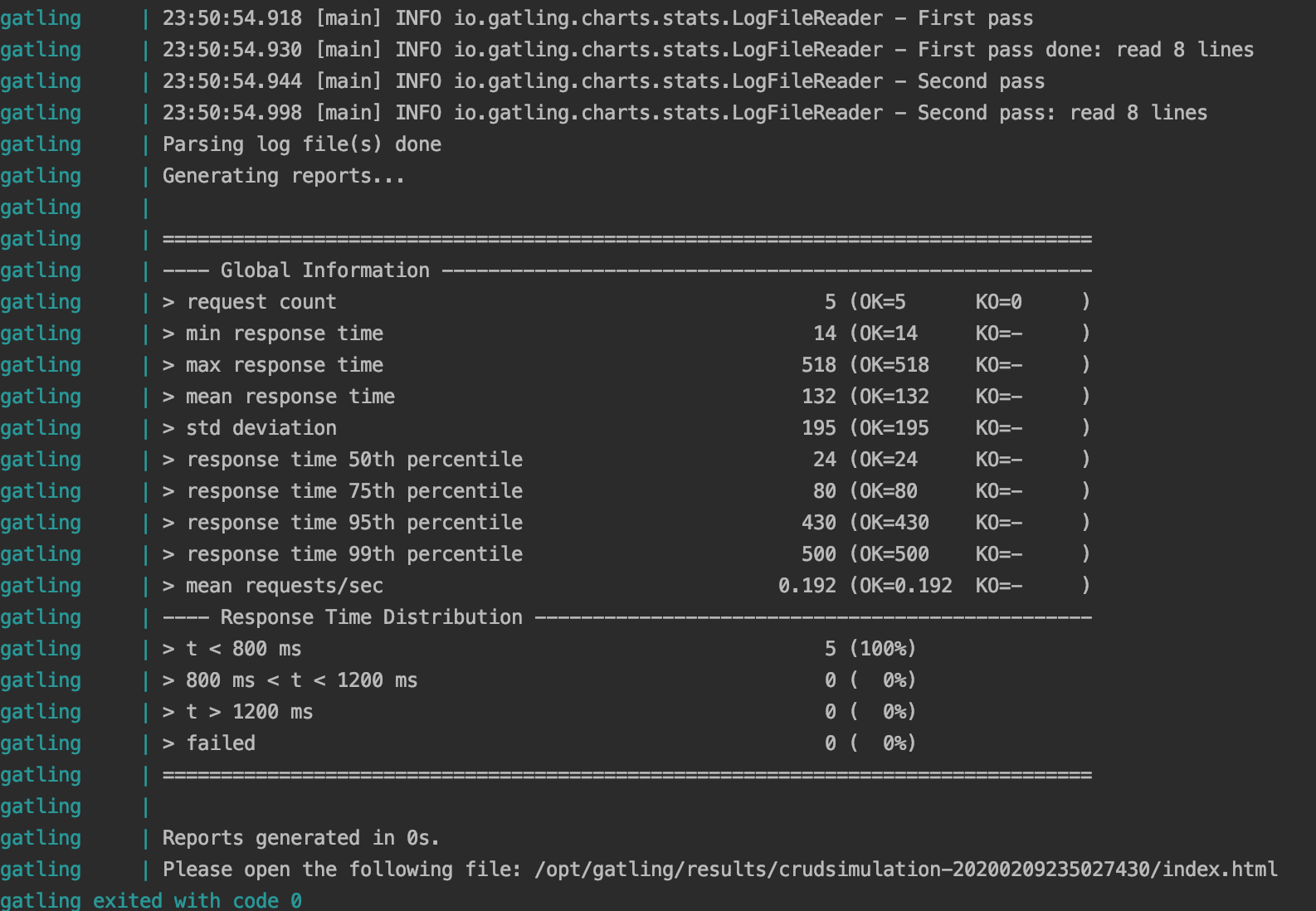


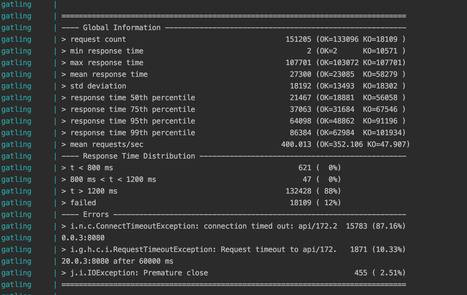 Now we got some errors! The cause, as we can see from the report, are timeouts from server threads been exhausted due to the massive amount of requests. In a real scenario, we should think of options such as horizontal balancing, reactive streams and such. But since our focus is not on API performance in the post, we will not continue for now. The main point for this little test is to show how Gatling can help us in testing the capacity of our applications.