

Welcome, dear reader! This is the last part of our series about the ELK stack, that provides a centralized architecture for gathering and analyse of application logs. On this last part, we will see how we can construct a rich front-end for our logging solution, using Kibana.
Kibana
Also developed by Elasticsearch, Kibana provides a way to explore the data and/or build rich dashboards of our data on the indexer. With a simple configuration, that consist of pointing Kibana to a ElasticSearch’s index – it also allows to point to multiple indexes at once, using a wildcard configuration -, it allow us to quickly set up a front-end for our stack.
So, without further delay, let’s begin our last step on the setup of our solution.
Hands-on
Installation
Beginning our lab, let’s download Kibana from the site. To do this, let’s open a terminal and type the following command:
curl https://download.elasticsearch.org/kibana/kibana/kibana-4.0.0-linux-x64.tar.gz | tar -zx
PS: this lab assumes the reader is using a linux 64-bit OS (I am using Ubuntu 14.10). If the reader is using another type of OS, the download page for Kibana is the following:
http://www.elasticsearch.org/overview/kibana/installation/
After running the command, we can see a folder called “kibana-4.0.0-linux-x64”. That’s all we need to do to install Kibana on our lab. Before we start running, however, we need to start both Logstash and ElasticSearch, to make our whole stack go live. If the reader didn’t have the stack set up, please refer to part 1 and part 2.
One configuration that the reader may take note is the elasticsearch_url property, inside the “kibana.yml” file, on the config folder. Since we didn’t change the default port from our elasticsearch’s cluster and we are running all the tools on the same machine, there is no need to change anything, but on a real world scenario, you may need to change this property to point to your elasticsearch’s cluster. The reader can made other configurations as well on this file, such as configuring a SSL connection between Kibana and Elasticsearch or configure the name of the index Kibana will use to store his metadata on elasticsearch.
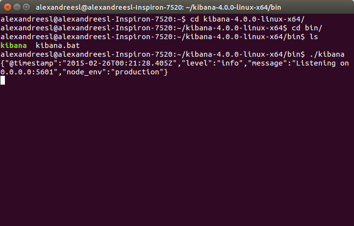
After we start the rest of the stack, it is time to run Kibana.To run it, we navigate to the bin folder of Kibana’s installation folder, and type:
./kibana
After some seconds, we can see that Kibana has successfully booted:
Set up
Now, let’s start using Kibana. Let’s open a web browser and enter:
On our first run, we will be greeted with the following screen:
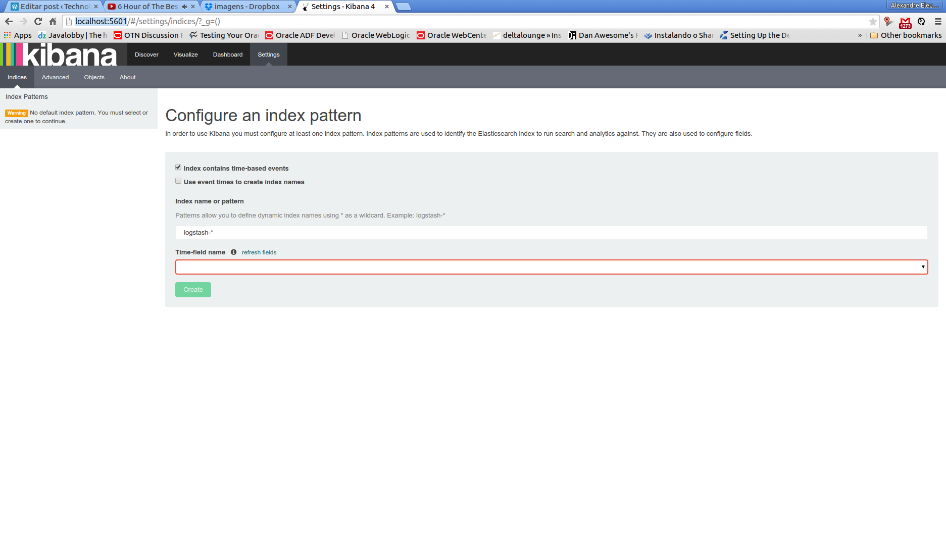
The reason because we are seeing this screen is because we dont have any index configured. It is on this screen that we can, for example, point to multiple indexes. If we think, for example, about the default naming pattern of logstash’s plugin, we can see that, for each new date we run, logstash will demand the creation of a new index with the pattern “logstash-%{+YYYY.MM.dd}”. So, if we want Kibana to use all the indexes created this way on a single dataset, we simply configure the field with the value “logstash-*”
On our case, we change the default naming of the index, to demonstrate the possible configurations of the tool, so we change the field to “log4jlogs”. One important thing to note on logstash’s plugin documentation, is that the idea behind the index pattern is to make more easy to do operations such as deleting old data, so in a real world scenario, it would be more wise to leave the default pattern enabled.
The other field we need to set is the Time-field name . This field is used by Kibana as a primary filter, allowing him to filter the data from the dashboards and data explorations on a timeline perspective. If we see our document type from the documents storing log information on elasticsearch, we can see it has a field called @timestamp. This field is perfectly fit to our time-field need, so we put “@timestamp” in the field.
After we click on the “create” button, we will be sent to a new page, where we can see all the fields from the index we pointed, proving that our configuration was a success:

Of course, there is other settings as well that we can configure, such as the precision on the numeric fields or the date mask when showing this kind of data on the interface, all available on the “advanced” menu. For our lab needs, however, the default options will suffice, so we leave this page by clicking on the “Discover” menu.
Discovering the data
When we enter the new page, if we didnt send any data to the cluster in the last 15 minutes, we will see a message of no data found (see bellow). The reason for this is because, by default, Kibana limits the results for the last 15 minutes only. To change this, we can either change the time limit by clicking on the value on the upper right corner of the page, or by running again the java program from the previous post, so we have more fresh data.

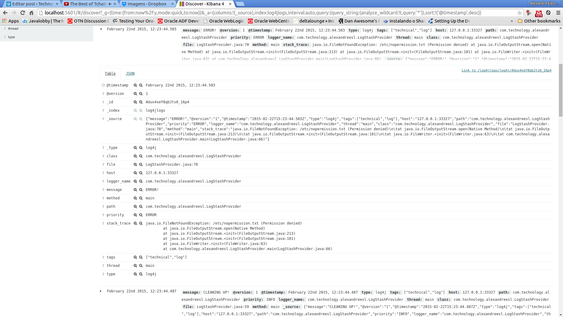
After we set some data to explore, we can see that the page changes to a data view, where we can dinamically change field filters, by changing the left menu, and drill down the data to the fields level, as we can see bellow. The reader can feel free to explore the page before we move on to our next part.
 Dashboards
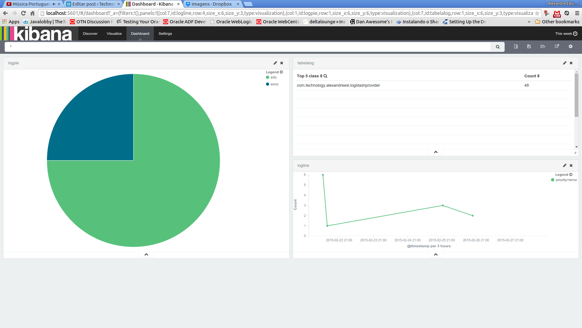
Now that we have all set, let’s begin by creating a simple dashboard. we will create a pie chart of the messages by the log level, a table view showing the count of messages by class and a line chart of the error messages across the time.
First, let’s begin with the pie chart. We will select, from the menu, “Visualize” , then follow this sequence of options on the next pages:
pie chart >> from a new search
We will enter a page like the one bellow:
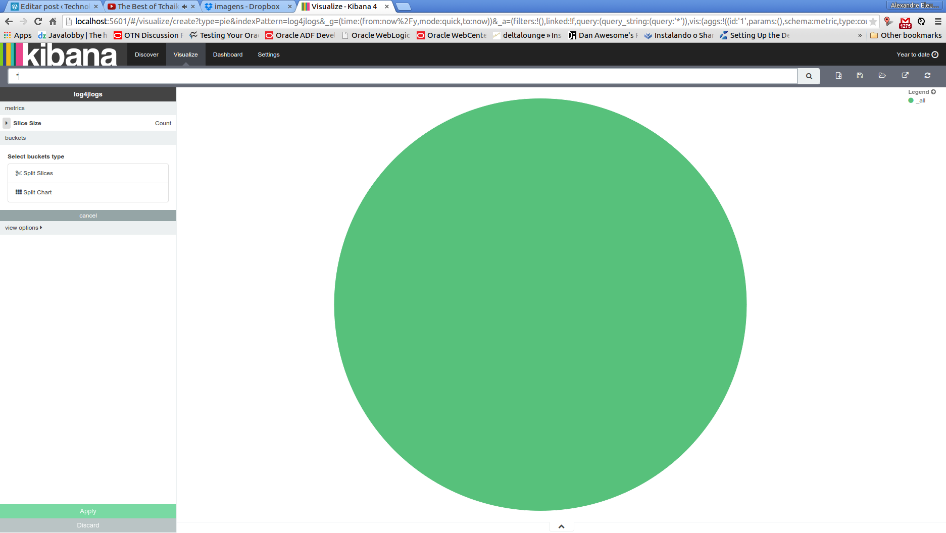
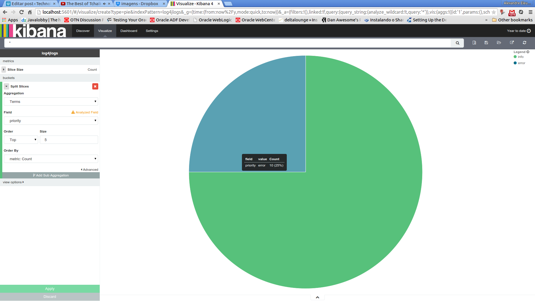
In this page, we will make our log level pie chart. To do this, we leave the metrics area unchanged, with the “count” value as slice size. Then, we choose “split slices” on the buckets area and select a “terms” aggregation, by the field “priority”. The screen bellow show our pie chart born!
After we made our chart, before we leave this page, we click on the disk icon on the top menu, input a name for our chart – also called visualization by Kibana’s terminology – and save it, for later use.
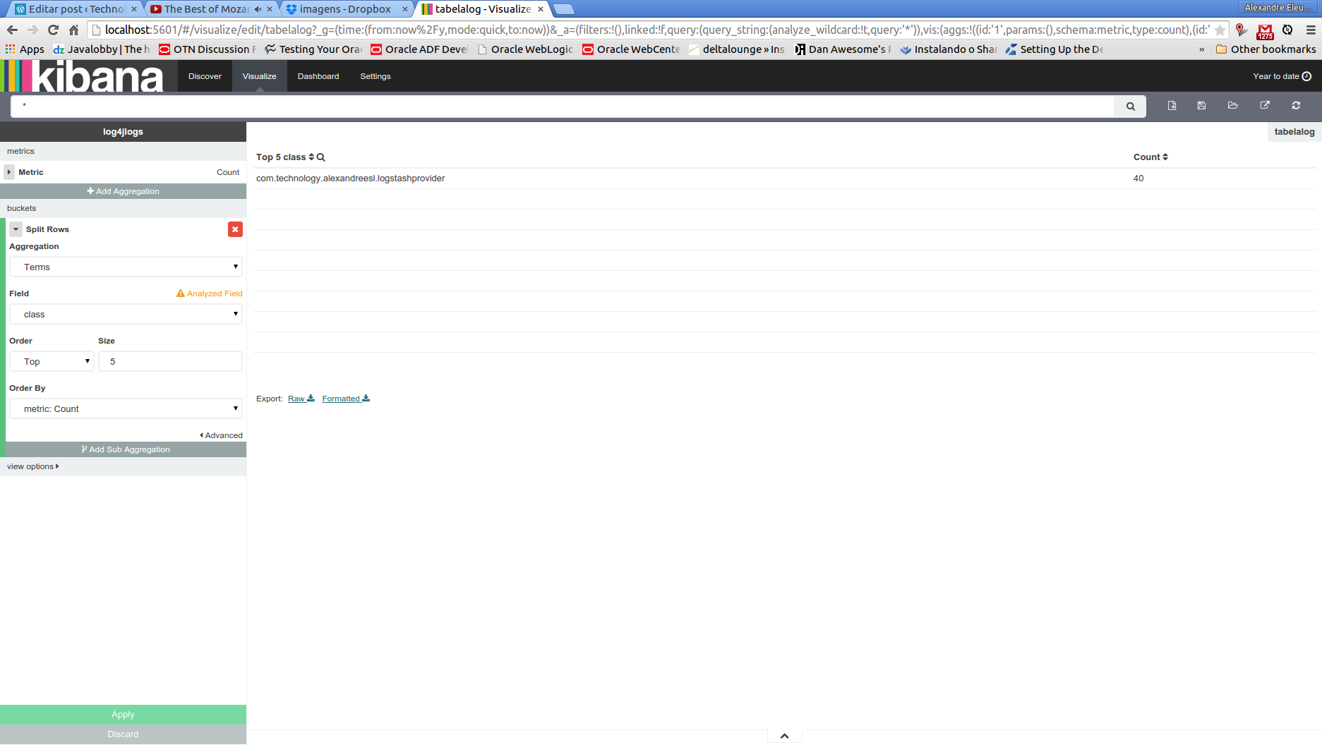
Now it is time for our table view. From the same menu we used to save our pie chart, click on the most left icon, called “new visualization”, then select “data table” and “from a new search”. We will see a similar page from the pie chart one, with similar options of aggregations and metrics to configure. With the intent of not bothering the reader with much repetitive instructions, from now on I will keep the explanation the more graphical possible, by the screenshots.
So, our data table view is made by making the configurations we can see on the left menu:
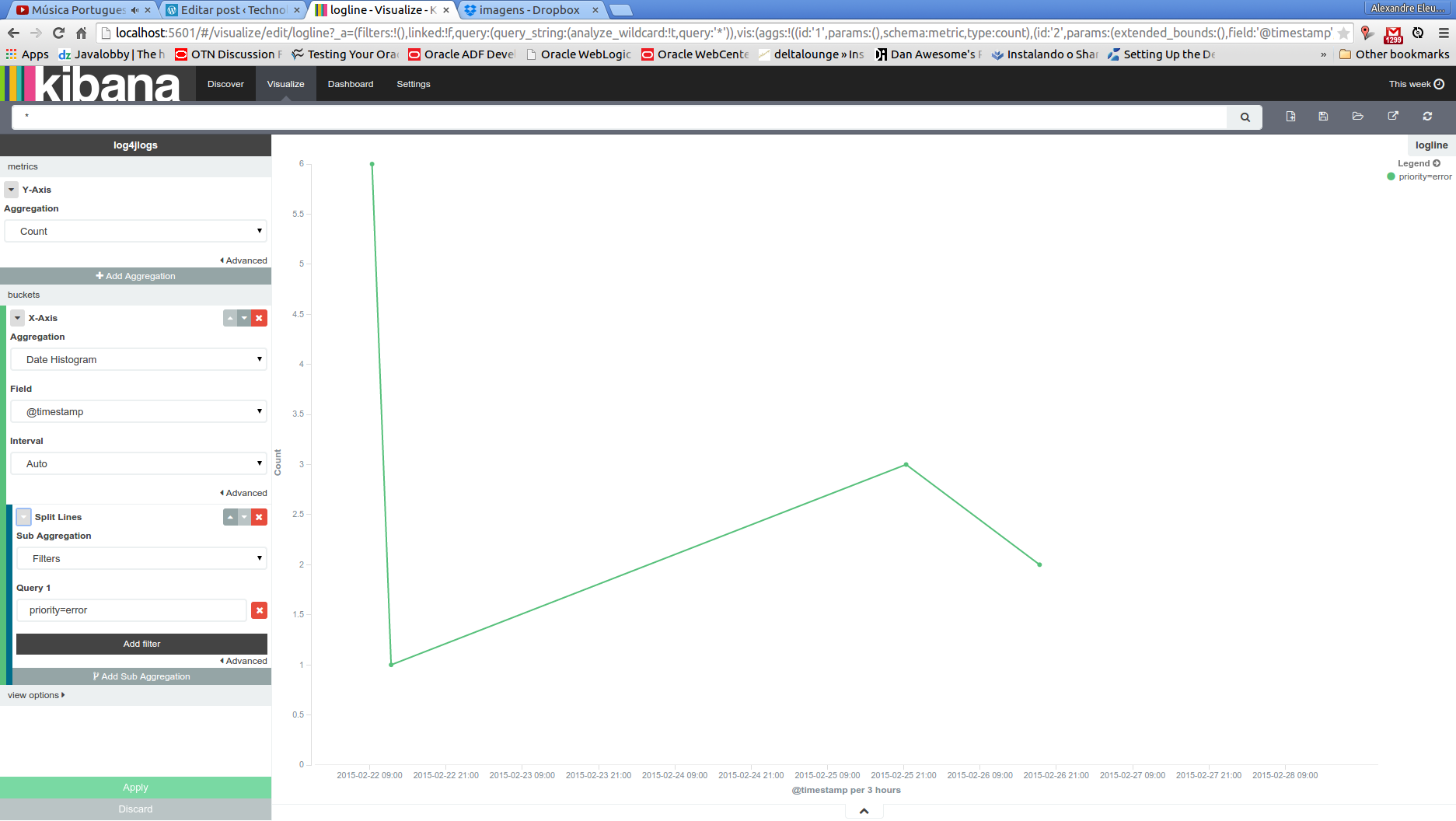
Analogous with what we made on the previous visualization, let’s also save the table view and click on new visualization, selecting line chart this time. The configuration for this chart can be seen bellow:
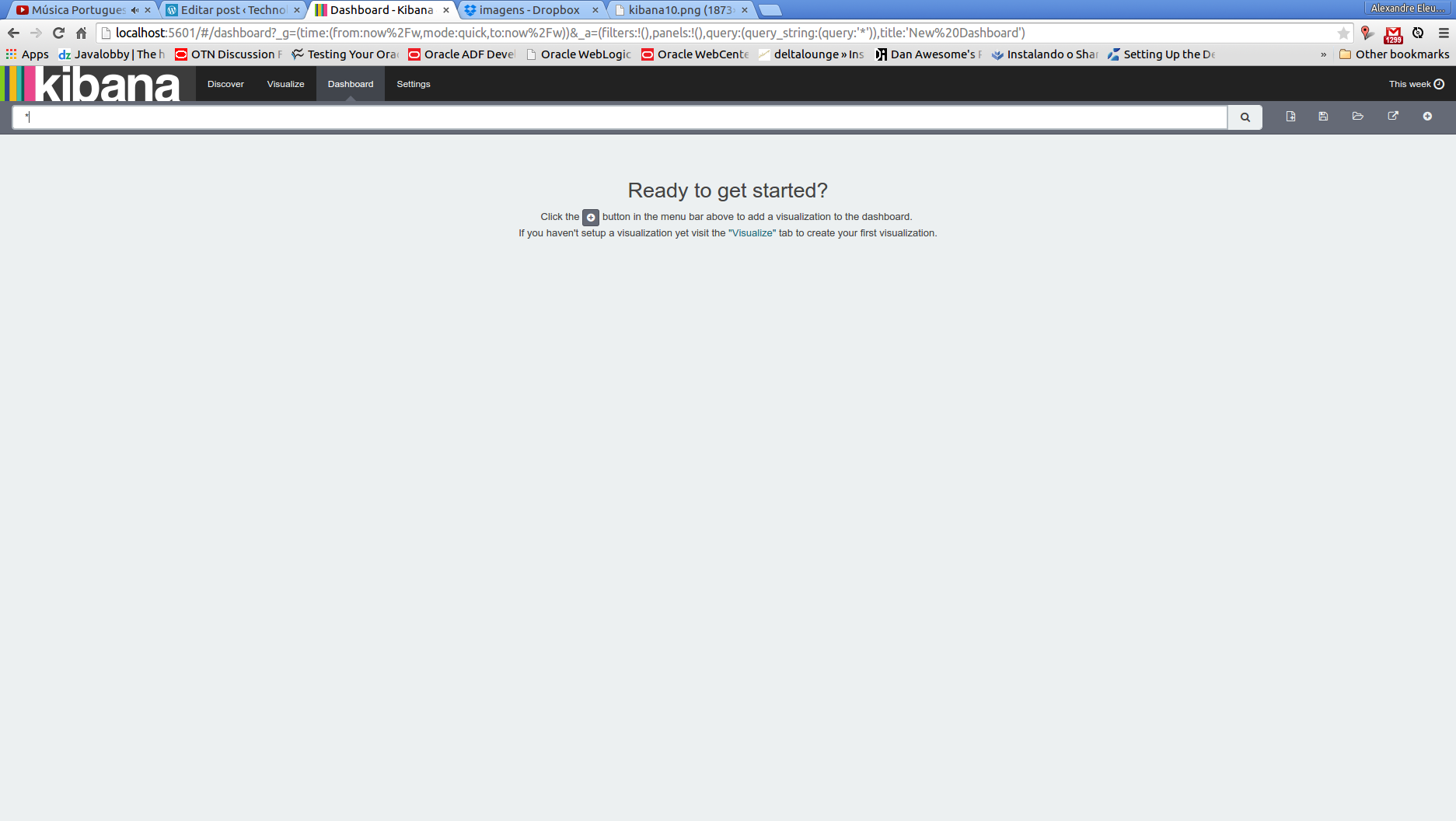
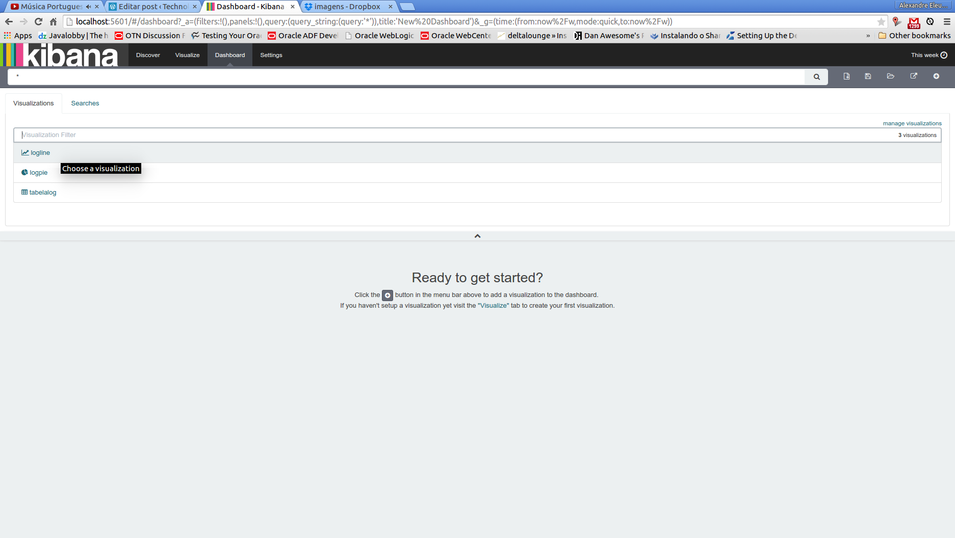
That concludes our visualizations. Now, let’s conclude our lab by making a dashboard that will show all the visualizations we build on the same page. To do this, first we select the “dashboard” option on the top menu. We will be greeted with the screen bellow:
This is the dashboard page, where we can create, edit and load dashboards. To add visualizations, we simply click on the plus icon on the top right side and select the visualization we want to add, like we can see bellow:
After we add the visualizations, it is pretty simple to arrange them: all we have to do is to drag and drop the visualizations as we like. My final arrangement of the dashboard is bellow, but the reader can arrange the way he finds best:
Finally, to save the dashboard, we simply click on the disk icon and input a name for our dashboard.
Cons
Of course, we cant make a complete overview of a tool, if we dont mention any noticeable con of it. The most visible downside of Kibana, on my opinion, is the lack of a native support to authentication and authorization. The reader may notice, by our tour of the interface, that there is no user or permission CRUDs whatsoever. Indeed, Kibana doesnt come with this feature.
One common workaround for this is to configure basic authentication on the web server Kibana runs with it – if we were using Kibana 3 on our lab, we would have to install manually a web server and deploy Kibana on it. On Kibana 4, we dont have to do this, because Kibana comes with a embedded node.js – , so the authentication is made by URL patterns. This link to the official node.js documentation provides a path to set basic authentication on the embedded server Kibana comes with it. The file that starts the server and need to be edited is on /src/bin/kibana.js.
Very recently, Elasticsearch has released shield, a plugin that implements a versatile security layer on Elasticsearch and subsequently on Kibana. Evidently, is a much more elegant and complete solution then the previous one, but the reader has to keep it in mind that he has to acquire a license to use shield.
Conclusion
And that concludes our tour by the ELK stack. Of course, on a real world scenario, we have some more steps to do, like the aforementioned authentication configuration, the configuration of purge policies and so on.However, we still can see that the core features we need were implemented, with very little effort. Like we talked about on the beginning of our series, logging information is a very rich source of information, that it has to be better explored on the business world. Thanks to everyone that follows my blog, until next time.

One thought on “ELK: using a centralized logging architecture – final part”