
Hello, dear readers! Welcome to my blog. On this post, we will talk about MongoDB aggregations, and how it could help us on developing powerful applications.
NoSQL
NoSQL (non-SQL) stands for databases that uses mechanisms that differ from traditional relational DBs. NoSQL DBs implement eventual consistency, which means there’s no read-after-write guarantee – but with clustering techniques, it is not typically a big deal – but with good clustering support, allows us to deploy robust databases with horizontal scalability and excellent performance, specially for data retrieval.
MongoDB
MongoDB is one of these databases that are classified as as NoSQL. It is document-based, meaning the data is stored as JSON-like objects (called BSONs, that internally are serialized as bytes to storage compression) in groups called collections, that are kind like tables in a database.
Used on thousands of companies across the globe, is one of the most popular NoSQL solutions around the world. It also provides a PAAS solution, called MongoDB Atlas.
Aggregations
Aggregations allows us to make operations upon data, like filtering, grouping, sums, counting, etc. At the end of the aggregation pipeline, we have our final, transformed, dataset with the results we want.
A good analogy to think about MongoDB aggregations is to imagine a conveyor belt in a factory. In this analogy, data are like parts been constructed in a factory: they got different construction stages, such as soldering, post manufactoring, etc. In the end, we have a finished part, ready to be shipped.
Now that we have the concepts effectively grasped, let’s begin to dive on the code!
Lab Setup
First, we need a dataset to make our aggregations. For this lab, we will use a dataset from fivethirtyeight, a popular site with public datasets for use in machine learning projects.
We will use a dataset containing lists of comic book characters from DC and Marvel up to 2014, compiled with their first appearance month/year and number of appearances since their debuts. The dataset is uploaded at the lab’s Github repository, and also can be found here.
The dataset comes in the format of two csv files. To import to MongoDB, we will use mongoimport. This link from Mongo’s documentation instruct how to install Mongo’s database tools.
We will use Docker to instantiate MongoDB database. In the repository we have a Docker Compose file ready to use to create the DB, by running:
docker-compose up -dAfter that, we can connect to Mongo using Mongo Shell, by typing:
mongoNext, let’s add the csvs to a new database called comic-book by inputing (from the project’s root folder):
mongoimport --db comic-book --collection DC --type csv --headerline --ignoreBlanks --file ./data/dc_wiki.csv
mongoimport --db comic-book --collection Marvel --type csv --headerline --ignoreBlanks --file ./data/marvel_wiki.csv
After running, in the shell, we can check everything was imported by running the following commands:
use comic-book
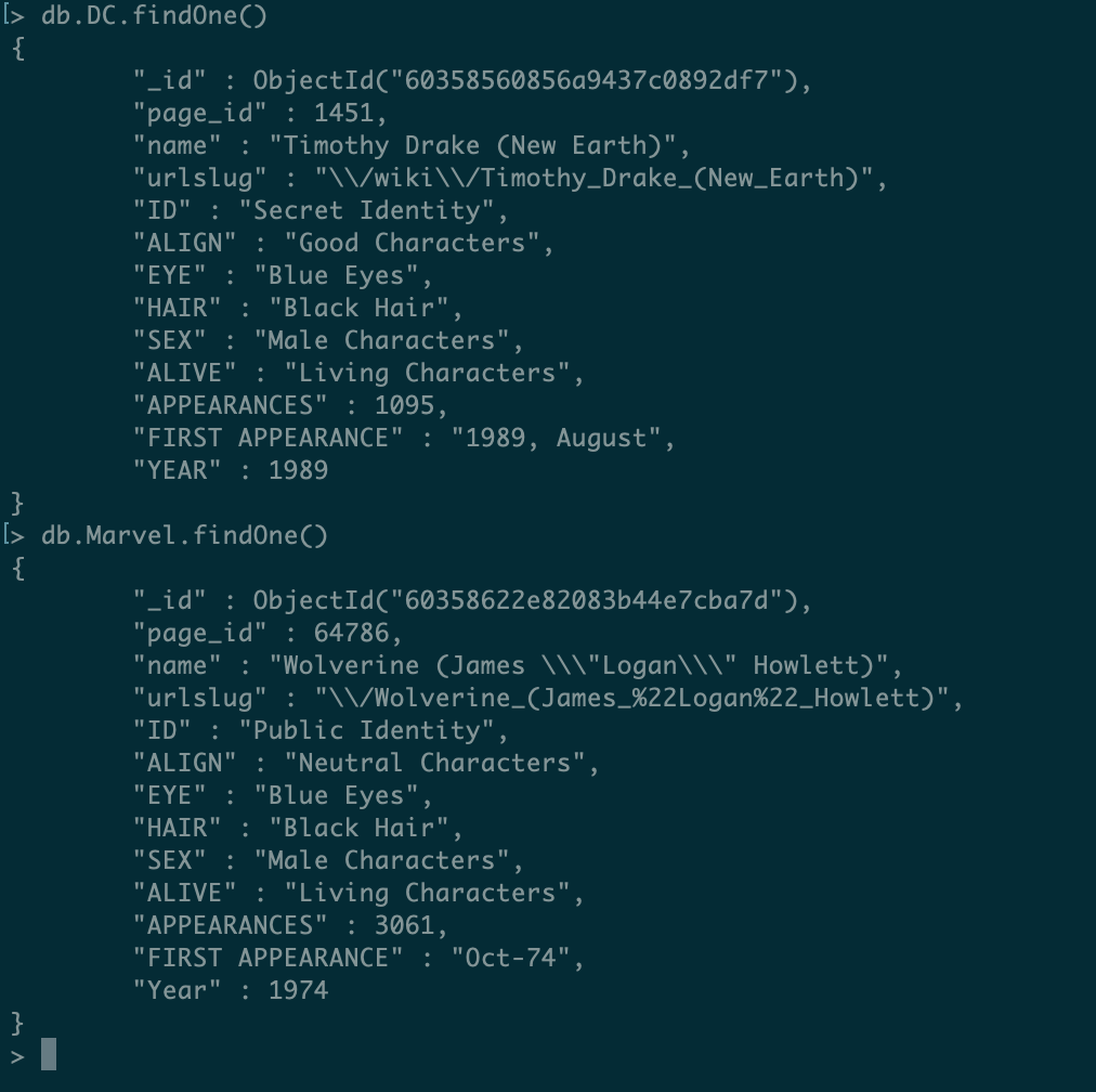
db.DC.findOne()
db.Marvel.findOne()This would produce results like the following:
Let’s now understanding the meaning of our dataset’s fields. As stated in the dataset’s repository, the fields are:
| Variable | Definition |
|---|---|
page_id | The unique identifier for that characters page within the wikia |
name | The name of the character |
urlslug | The unique url within the wikia that takes you to the character |
ID | The identity status of the character (Secret Identity, Public identity, [on marvel only: No Dual Identity]) |
ALIGN | If the character is Good, Bad or Neutral |
EYE | Eye color of the character |
HAIR | Hair color of the character |
SEX | Sex of the character (e.g. Male, Female, etc.) |
GSM | If the character is a gender or sexual minority (e.g. Homosexual characters, bisexual characters) |
ALIVE | If the character is alive or deceased |
APPEARANCES | The number of appareances of the character in comic books (as of Sep. 2, 2014. Number will become increasingly out of date as time goes on.) |
FIRST APPEARANCE | The month and year of the character’s first appearance in a comic book, if available |
YEAR | The year of the character’s first appearance in a comic book, if available |
Now that we have our data ready, let’s begin aggregating!
Our first aggregations
For this lab, we will use Python 3.6. As a first example, let’s search for all Flashes there is on DC comics. For this, we create a generic runner structure, composed of a main script:
import re

from aggregations.aggregations import run


def main():
    run('DC', [{
        '$match': {
            'name': re.compile(r"Flash")
        }
    }])


if __name__ == "__main__":
    main()
And a generic aggregation runner, where we pass the pipeline to be executed as a parameter:
from pymongo import MongoClient
import pprint

client = MongoClient('mongodb://localhost:27017/?readPreference=primary&appname=MongoDB%20Compass&ssl=false')


def run(collection, pipeline):
    result = client['comic-book'][collection].aggregate(
        pipeline
    )

    pprint.pprint(list(result))
After running it, we will get the following results:
[{'ALIGN': 'Good Characters',
  'ALIVE': 'Living Characters',
  'APPEARANCES': 1028,
  'EYE': 'Blue Eyes',
  'FIRST APPEARANCE': '1956, October',
  'HAIR': 'Blond Hair',
  'ID': 'Secret Identity',
  'SEX': 'Male Characters',
  'YEAR': 1956,
  '_id': ObjectId('60358560856a9437c0892dfa'),
  'name': 'Flash (Barry Allen)',
  'page_id': 1380,
  'urlslug': '\\/wiki\\/Flash_(Barry_Allen)'},
 {'ALIGN': 'Good Characters',
  'ALIVE': 'Living Characters',
  'APPEARANCES': 14,
  'FIRST APPEARANCE': '2008, August',
  'SEX': 'Male Characters',
  'YEAR': 2008,
  '_id': ObjectId('60358560856a9437c08934ac'),
  'name': 'Well-Spoken Sonic Lightning Flash (New Earth)',
  'page_id': 87335,
  'urlslug': '\\/wiki\\/Well-Spoken_Sonic_Lightning_Flash_(New_Earth)'},
 {'ALIGN': 'Neutral Characters',
  'ALIVE': 'Living Characters',
  'APPEARANCES': 12,
  'FIRST APPEARANCE': '1998, June',
  'SEX': 'Male Characters',
  'YEAR': 1998,
  '_id': ObjectId('60358560856a9437c08935ac'),
  'name': 'Black Flash (New Earth)',
  'page_id': 22026,
  'urlslug': '\\/wiki\\/Black_Flash_(New_Earth)'},
 {'ALIGN': 'Bad Characters',
  'ALIVE': 'Living Characters',
  'APPEARANCES': 3,
  'FIRST APPEARANCE': '2007, November',
  'ID': 'Secret Identity',
  'SEX': 'Male Characters',
  'YEAR': 2007,
  '_id': ObjectId('60358560856a9437c0893f36'),
  'name': 'Bizarro Flash (New Earth)',
  'page_id': 32435,
  'urlslug': '\\/wiki\\/Bizarro_Flash_(New_Earth)'},
 {'ALIGN': 'Good Characters',
  'ALIVE': 'Living Characters',
  'EYE': 'Green Eyes',
  'FIRST APPEARANCE': '1960, January',
  'HAIR': 'Red Hair',
  'ID': 'Secret Identity',
  'SEX': 'Male Characters',
  'YEAR': 1960,
  '_id': ObjectId('60358560856a9437c08948d3'),
  'name': 'Flash (Wally West)',
  'page_id': 1383,
  'urlslug': '\\/wiki\\/Flash_(Wally_West)'}]
Lol, that’s a lot of Flashes! However, we also got some villains together, such as the strange Bizarro Flash. let’s improve our pipeline by filtering to only show the good guys:
[{
        '$match': {
            'name': re.compile(r"Flash ", flags=re.IGNORECASE),
            'ALIGN': 'Good Characters'
        }
    }]
If we run again, we can see characters such as Bizarro Flash no longer exist in our results.
We also had our first glance at our first pipeline stage, $match. This stage allows us to filter our results, by using the same kind of filtering expressions we can use in normal searches.
In MongoDB’s aggregations, an aggregation pipeline is composed of stages, which are the items inside an array that will be executed by Mongo. The stages are executed from first to last item in the array, with the output of one stage servings as input for the next.
As an example of how a pipeline can have multiple stages and how each stage handles the data from the previous one, let’s use another stage, $project. Project allows us to create new fields by applying operations to it (more in a minute) and also allow us to control which fields we want on our results. Let’s remove all other fields except for the name and first appearance to see this in practice:
[{
        '$match': {
            'name': re.compile(r"Flash ", flags=re.IGNORECASE),
            'ALIGN': 'Good Characters'
        }
    },
    {
        '$project': {
            'FIRST APPEARANCE': 1, 'name': 1, '_id': 0
        }
    }]
When defining which fields to maintain, we use 1 to define a field to be maintained and 0 to define fields that won’t be maintained (only the defined fields will be maintained, the only field we need to use 0 to define we don’t want is the object’s ID field, so we set 0 only for him).
This produces the following:
[{'FIRST APPEARANCE': '1956, October', 'name': 'Flash (Barry Allen)'},
 {'FIRST APPEARANCE': '2008, August',
  'name': 'Well-Spoken Sonic Lightning Flash (New Earth)'},
 {'FIRST APPEARANCE': '1960, January', 'name': 'Flash (Wally West)'}]
Now, let’s make another aggregation. In our dataset, the first appearance is a string following this pattern:
<year> , <month>Not only that, we also have some “dirty” data, as there is records without this field, or records with just the year in numerical format. We need to do some cleaning, using just characters we have the information and transform the data to a standard numerical field, in order to make it more useful for our use cases.
Now, let’s say we want to know the names of all characters created in the comics silver age (a time-period that goes from 1956 to 1970). To do this, first we create a field with the first appearance’s year, like we said before, and then use the new field to filter only silver age characters.
We already have a field with the year properly defined on the dataset, but for exercise’s sake, let’s suppose we had only this string-formatted field available, in order to examine more features and simulate real-world scenarios where many times data has formatting and correctness issues.
Let’s begin by creating our new field:
[
        {
        '$match': {
            'FIRST APPEARANCE': {'$exists': True}
        }
        },
        {
            '$project': {
                '_id': 0,
                'name': 1,
                'year': {'$toInt': {'$arrayElemAt': [{'$split': [{'$toString': '$FIRST APPEARANCE'}, ","]}, 0]}}
            }
        }
    ]
Lol, that’s some transforming! We filter the records to just use the ones that have the field, and in project stage we make conversions to allows us to extract the year from the field and convert him to a number. This produces something like this fragment:
 ...
 {'name': 'Tempus (New Earth)', 'year': 1997},
 {'name': 'Valkyra (New Earth)', 'year': 1997},
 {'name': 'Spider (New Earth)', 'year': 1997},
 {'name': 'Vayla (New Earth)', 'year': 1997},
 {'name': 'Widow (New Earth)', 'year': 1997},
 {'name': "William O'Neil (New Earth)", 'year': 1997},
 {'name': 'Arzaz (New Earth)', 'year': 1996},
 {'name': 'Download II (New Earth)', 'year': 1996}
...
With everything transformed, we only need to filter the year to get our silver age characters:
        [{
            '$match': {
                'FIRST APPEARANCE': {'$exists': True}
            }
        },
        {
            '$project': {
                '_id': 0,
                'name': 1,
                'year': {'$toInt': {'$arrayElemAt': [{'$split': [{'$toString': '$FIRST APPEARANCE'}, ","]}, 0]}}
            }
        },
        {
            '$match': {
                'year': {"$gte": 1956, "$lte": 1970}
            }
        }]
This produces the following list (just a fragment, due to size):
[{'name': 'Dinah Laurel Lance (New Earth)', 'year': 1969},
 {'name': 'Flash (Barry Allen)', 'year': 1956},
 {'name': 'GenderTest', 'year': 1956},
 {'name': 'Barbara Gordon (New Earth)', 'year': 1967},
 {'name': 'Green Lantern (Hal Jordan)', 'year': 1959},
 {'name': 'Raymond Palmer (New Earth)', 'year': 1961},
 {'name': 'Guy Gardner (New Earth)', 'year': 1968},
 {'name': 'Garfield Logan (New Earth)', 'year': 1965},
 {'name': 'Ralph Dibny (New Earth)', 'year': 1960},
...
Talking about big lists, one feature that is good to keep in mind when aggregating datasets, is that there is a memory limit imposed by MongoDB for doing in-memory aggregation (the default behavior). To allow MongoDB to use disk swap when aggregating, we add the following option when running the pipeline:
result = client['comic-book'][collection].aggregate(
        pipeline, allowDiskUse=True
    )
By running again, we can see everything is still working as expected.
We also can notice the results are not sorted. To sort by the name, we can add a $sort stage:
        [{
            '$match': {
                'FIRST APPEARANCE': {'$exists': True}
            }
        },
        {
            '$project': {
                '_id': 0,
                'name': 1,
                'year': {'$toInt': {'$arrayElemAt': [{'$split': [{'$toString': '$FIRST APPEARANCE'}, ","]}, 0]}}
            }
        },
        {
            '$match': {
                'year': {"$gte": 1956, "$lte": 1970}
            }
        },
        {
            '$sort': {
                'name': 1
            }
        }]
The $sort stage receives fields definitions, where 1 means ascending order and -1 means descending. After running, we can see the results were sorted:
[{'name': 'Abel (New Earth)', 'year': 1969},
 {'name': 'Abel Tarrant (New Earth)', 'year': 1963},
 {'name': 'Abin Sur (New Earth)', 'year': 1959},
 {'name': 'Abnegazar (New Earth)', 'year': 1962},
 {'name': 'Abner Krill (New Earth)', 'year': 1962},
 {'name': 'Ace Arn (New Earth)', 'year': 1965},
 {'name': 'Ace Chance (New Earth)', 'year': 1966},
 {'name': 'Achilles Milo (New Earth)', 'year': 1957},
 {'name': 'Adam Strange (New Earth)', 'year': 1958},
 {'name': 'Agantha (New Earth)', 'year': 1964},
 {'name': 'Ahk-Ton (New Earth)', 'year': 1965},
 {'name': 'Alanna Strange (New Earth)', 'year': 1958},
 {'name': 'Albert Desmond (New Earth)', 'year': 1958},
 {'name': 'Albrecht Raines (New Earth)', 'year': 1958},
 {'name': 'Alpheus Hyatt (New Earth)', 'year': 1962},
 {'name': 'Aluminum (New Earth)', 'year': 1963},
 {'name': 'Amazo (New Earth)', 'year': 1960},
 {'name': 'Amos Fortune (New Earth)', 'year': 1961},
 {'name': 'Anais Guillot (New Earth)', 'year': 1959},
...
Now, let’s suppose we just wanted to count how many characters from silver age are on DC, not know their names or any other data. We could do this by adding a $count stage:
[{
            '$match': {
                'FIRST APPEARANCE': {'$exists': True}
            }
        },
        {
            '$project': {
                '_id': 0,
                'name': 1,
                'year': {'$toInt': {'$arrayElemAt': [{'$split': [{'$toString': '$FIRST APPEARANCE'}, ","]}, 0]}}
            }
        },
        {
            '$match': {
                'year': {"$gte": 1956, "$lte": 1970}
            }
        },
        {
            '$count': 'total'
        }]
Count only ask us to define a name for the count. This would produce the following:
[{'total': 556}]Grouping data together
Let’s start using Marvel collection now. To know how many characters there are in Marvel according to their aligns (neutral, good or bad), we use a $group stage to group the data by the align and use a accumulator to count the characters:
[
        {
            '$match': {
                'ALIGN': {'$exists': True}
            }
        },
        {
            '$group': {
                '_id': '$ALIGN',
                'count': {'$sum': 1}
            }
        }
    ]
Yes, is simple as that! This produces the following:
[{'_id': 'Good Characters', 'count': 4636},
 {'_id': 'Bad Characters', 'count': 6720},
 {'_id': 'Neutral Characters', 'count': 2208}]
Now, let’s try a different example. We want to count all characters created by Marvel, breaking down by decade.
To make this grouping, we will use the $bucket stage, as follows:
[{
            '$bucket': {
                'groupBy': "$Year",
                'boundaries': [1930, 1940, 1950, 1960, 1970, 1980, 1990, 2000, 2010, 2020],
                'default': "Unknown",
                'output': {
                    'count': {'$sum': 1}
                }
            }
        }]
Here we have a groupBy field to define which field to use as bucket selector. We define boundaries for the buckets and a default in case a bucket can’t be defined. Finally, we have an output, where we define aggregators to be executed for each bucket.
This produces the following results:
[{'_id': 1930, 'count': 69},
 {'_id': 1940, 'count': 1441},
 {'_id': 1950, 'count': 302},
 {'_id': 1960, 'count': 1306},
 {'_id': 1970, 'count': 2234},
 {'_id': 1980, 'count': 2425},
 {'_id': 1990, 'count': 3657},
 {'_id': 2000, 'count': 3086},
 {'_id': 2010, 'count': 1041},
 {'_id': 'Unknown', 'count': 815}]
Another type of bucketing is by using the $bucketAuto stage. This stage allows us to let MongoDB do the grouping for us, without needing to define the boundaries. Let’s try it out with DC:
[{
            '$bucketAuto': {
                'groupBy': "$YEAR",
                'buckets': 10,
                'output': {
                    'count': {'$sum': 1}
                }
            }
        }]
This produces:
[{'_id': {'max': 1965, 'min': None}, 'count': 702},
 {'_id': {'max': 1981, 'min': 1965}, 'count': 703},
 {'_id': {'max': 1987, 'min': 1981}, 'count': 779},
 {'_id': {'max': 1990, 'min': 1987}, 'count': 806},
 {'_id': {'max': 1994, 'min': 1990}, 'count': 707},
 {'_id': {'max': 1998, 'min': 1994}, 'count': 779},
 {'_id': {'max': 2004, 'min': 1998}, 'count': 791},
 {'_id': {'max': 2008, 'min': 2004}, 'count': 752},
 {'_id': {'max': 2011, 'min': 2008}, 'count': 716},
 {'_id': {'max': 2013, 'min': 2011}, 'count': 161}]
By default, Mongo will try to spread the buckets the more evenly as possible. We can define a field called granularity to better restrict how we want to group:
[{
            '$match': {
                'YEAR': {'$exists': True}
            }
        },
        {
            '$bucketAuto': {
                'groupBy': '$YEAR',
                'buckets': 10,
                'granularity': 'E192',
                'output': {
                    'count': {'$sum': 1}
                }
            }
        }]
This defines a preferred time series to round the buckets and calculate the edges. More info can be found at the documentation. One important thing to note is that granularity must only be used on numeric buckets and must not contain data without the field (that’s why we introduced the filter).
This produces:
[{'_id': {'max': 1980.0, 'min': 1930.0}, 'count': 1300},
 {'_id': {'max': 2000.0, 'min': 1980.0}, 'count': 3429},
 {'_id': {'max': 2030.0, 'min': 2000.0}, 'count': 2098}]
Faceting & persisting the results
Now, let’s make a report where we have some of our previous aggregations grouped in a single result, like a report. We can do this by creating facet stages, which act like independent pipelines that will be grouped as a single result at the end.
This can be achieved by adding the following facets:
[
        {
            '$facet': {
                'Silver age characters': [
                    {
                        '$match': {
                            'FIRST APPEARANCE': {'$exists': True}
                        }
                    },
                    {
                        '$project': {
                            '_id': 0,
                            'name': 1,
                            'year': {
                                '$toInt': {'$arrayElemAt': [{'$split': [{'$toString': '$FIRST APPEARANCE'}, ","]}, 0]}}
                        }
                    },
                    {
                        '$match': {
                            'year': {"$gte": 1956, "$lte": 1970}
                        }
                    },
                    {
                        '$sort': {
                            'name': 1
                        }
                    }
                ],
                'Characters by decade': [
                    {
                        '$bucket': {
                            'groupBy': "$YEAR",
                            'boundaries': [1930, 1940, 1950, 1960, 1970, 1980, 1990, 2000, 2010, 2020],
                            'default': "Unknown",
                            'output': {
                                'count': {'$sum': 1}
                            }
                        }
                    }
                ]
            }
        }
    ]
This produces results like the following, running for DC:
[{'Characters by decade': [{'_id': 1930, 'count': 42},
                           {'_id': 1940, 'count': 268},
                           {'_id': 1950, 'count': 121},
                           {'_id': 1960, 'count': 453},
                           {'_id': 1970, 'count': 416},
                           {'_id': 1980, 'count': 1621},
                           {'_id': 1990, 'count': 1808},
                           {'_id': 2000, 'count': 1658},
                           {'_id': 2010, 'count': 440},
                           {'_id': 'Unknown', 'count': 69}],
  'Silver age characters': [{'name': 'Abel (New Earth)', 'year': 1969},
                            {'name': 'Abel Tarrant (New Earth)', 'year': 1963},
                            {'name': 'Abin Sur (New Earth)', 'year': 1959},
                            {'name': 'Abnegazar (New Earth)', 'year': 1962},
                            {'name': 'Abner Krill (New Earth)', 'year': 1962},
                            {'name': 'Ace Arn (New Earth)', 'year': 1965},
...
Now, what if we wanted to persist this report, without having to resort to -re-run the aggregation? For this, we add a $out stage, which persist the aggregation’s results on a collection. Let’s change our pipeline like this:
[
        {
            '$facet': {
                'Silver age characters': [
                    {
                        '$match': {
                            'FIRST APPEARANCE': {'$exists': True}
                        }
                    },
                    {
                        '$project': {
                            '_id': 0,
                            'name': 1,
                            'year': {
                                '$toInt': {'$arrayElemAt': [{'$split': [{'$toString': '$FIRST APPEARANCE'}, ","]}, 0]}}
                        }
                    },
                    {
                        '$match': {
                            'year': {"$gte": 1956, "$lte": 1970}
                        }
                    },
                    {
                        '$sort': {
                            'name': 1
                        }
                    }
                ],
                'Characters by decade': [
                    {
                        '$bucket': {
                            'groupBy': "$YEAR",
                            'boundaries': [1930, 1940, 1950, 1960, 1970, 1980, 1990, 2000, 2010, 2020],
                            'default': "Unknown",
                            'output': {
                                'count': {'$sum': 1}
                            }
                        }
                    }
                ]
            }
        },
        {'$out': 'DC-reports'}
    ]
After running, we can check the DB for the persisted data:
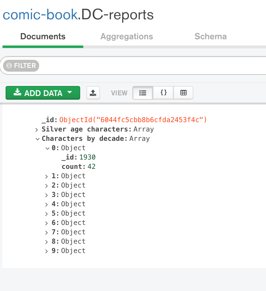
IMPORTANT: All data on the collection will be deleted and replaced by the aggregation’s results upon re-running!
Conclusion
And that concludes our quick tour on MongoDB’s aggregations. Of course, this is just a taste of what we are capable of with the framework. I suggest reading the documentation for learning more features, such as $lookup, that allows us to left-join collections.
With a simple and intuitive interface, is a very robust and powerful solution, that must be explored. Thank you for following me on one more article, until next time.